Your browser does not fully support modern features. Please upgrade for a smoother experience.
Submitted Successfully!
 +1 credit
Thank you for your contribution! You can also upload a video entry or images related to this topic.
For video creation, please contact our Academic Video Service.
| Version | Summary | Created by | Modification | Content Size | Created at | Operation |
|---|---|---|---|---|---|---|
| 1 | Daniel A. Griffith | -- | 1497 | 2023-09-28 20:22:39 | | | |
| 2 | Catherine Yang | Meta information modification | 1497 | 2023-10-07 10:42:45 | | |
Video Upload Options
We provide professional Academic Video Service to translate complex research into visually appealing presentations. Would you like to try it?
Cite
If you have any further questions, please contact Encyclopedia Editorial Office.
Griffith, D.A. Understanding Spatial Autocorrelation. Encyclopedia. Available online: https://encyclopedia.pub/entry/49783 (accessed on 24 June 2026).
Griffith DA. Understanding Spatial Autocorrelation. Encyclopedia. Available at: https://encyclopedia.pub/entry/49783. Accessed June 24, 2026.
Griffith, Daniel A.. "Understanding Spatial Autocorrelation" Encyclopedia, https://encyclopedia.pub/entry/49783 (accessed June 24, 2026).
Griffith, D.A. (2023, September 28). Understanding Spatial Autocorrelation. In Encyclopedia. https://encyclopedia.pub/entry/49783
Griffith, Daniel A.. "Understanding Spatial Autocorrelation." Encyclopedia. Web. 28 September, 2023.
Copy Citation
An enumeration of spatial autocorrelation’s (SA’s) polyvalent forms occurred nearly three decades ago. Attempts to conceive and disseminate a clearer explanation of it employ metaphors seeking to better relate SA to a student’s or spatial scientist’s personal knowledge databank.
Moran scatterplot
negative spatial autocorrelation
positive spatial autocorrelation
1. Introduction
Salvati [1] points out that “evidence from the analysis of scientific databanks and repositories indicates how the geography discipline has a strong potential for growth and [facilitating] the dissemination of complex global problems.” Realizing this potential requires a wider awareness and deeper understanding of an often glossed over, ignored, or unschooled fundamental property of all of the geospatial data housed in the databanks and repositories he mentions, namely, spatial autocorrelation (SA)—the tendency for (dis)similar attribute values to cluster on a map. As Griffith [2] professes, SA is everywhere! Accordingly, it is an essential ingredient for “develop[ing] and offer[ing] new strategies, visions and proposals on the role of sustainability and resilience related to urban and rural contexts” [1], such as partially constituting the spatial statistical theory underlying tessellated stratified random sampling necessary for economically and efficiently monitoring and “studying [the] degree of resilience and future (sustainable) development [of large territories]” [1]. Not only is SA a fundamental property of georeferenced data, but it also is a fundamental geographic concept (e.g., Tobler’s [3] First Law of Geography; see https://www.researchgate.net/publication/276917830_Concepts_and_Principles_for_Spatial_Literacy (accessed on 24 August 2023)). Its history dates back to its informal, tacit, non-verbal awareness concept formation recognition by, for example, Spilsbury in 1767 [4], who invented the jigsaw puzzle to teach geography, and Brandes in 1816 [5], who invented the isobar map to visualize general west-to-east movements of low pressure across Europe. Nearly a century later, SA had its formal concept creation recognition by Student [6], followed by a quarter century of acknowledgements about its correlated data source [7][8][9] and its impacts on agricultural experimental designs [10][11], its quantification by Moran [12] and Geary [13], its popularization by Cliff and Ord [14], as well as Journel and Huijbregts [15], and its promotion as part of standard spatial statistical/econometric practice by Paelinck and Klaassen [16], Anselin [17], Cressie [18], and Haining [19], among others.
The concept of SA may be more meticulously defined as follows:
Coupling a tertile-classified set of attribute values [i.e., relatively high (H), intermediate (M), and relatively low (L) magnitude groups] with a posited geographic neighbors definition (e.g., nearby points, adjacent line segments, and/or juxtaposed polygons sharing a non-zero length common boundary—the rook designation, based upon its resemblance to chess piece moves), the tendency for pairs of H, of M, and/or of L values (positive SA), or the tendency for contrasting high-low (H-L) or low-high (L-H) value pairings as well as still pairs of M values (negative SA), to be neighbors as defined by this given geographic-based construction.
This tertile definition builds upon Anselin’s [20] local SA index conceptualization, which translates points in a Moran scatterplot into neighboring pairings denoted by high-high (H-H), low-low (L-L), H-L, and L-H; insignificant areal units constitute the M values. SA has other correlated data parallels, including those involving matched pairs, time series, space-time series, and network series [21].
During its catapulting into the forefront of the quantitative spatial sciences, many students, in particular, of quantitative geography found understanding SA and its consequences a challenge, spawning a set of earlier publications devoted to explicating it [22][23]; Griffith also published a monograph with this title in 1987). Contemporary literature, including Getis [24], Goodchild [25], Griffith [26], Haining [27], Legendre [28], and McMillan [29], contains a number of standalone explanatory treatments of SA. Today, the body of literature dedicated to SA is sizeable (Figure 1; for an updated version, see [30]).
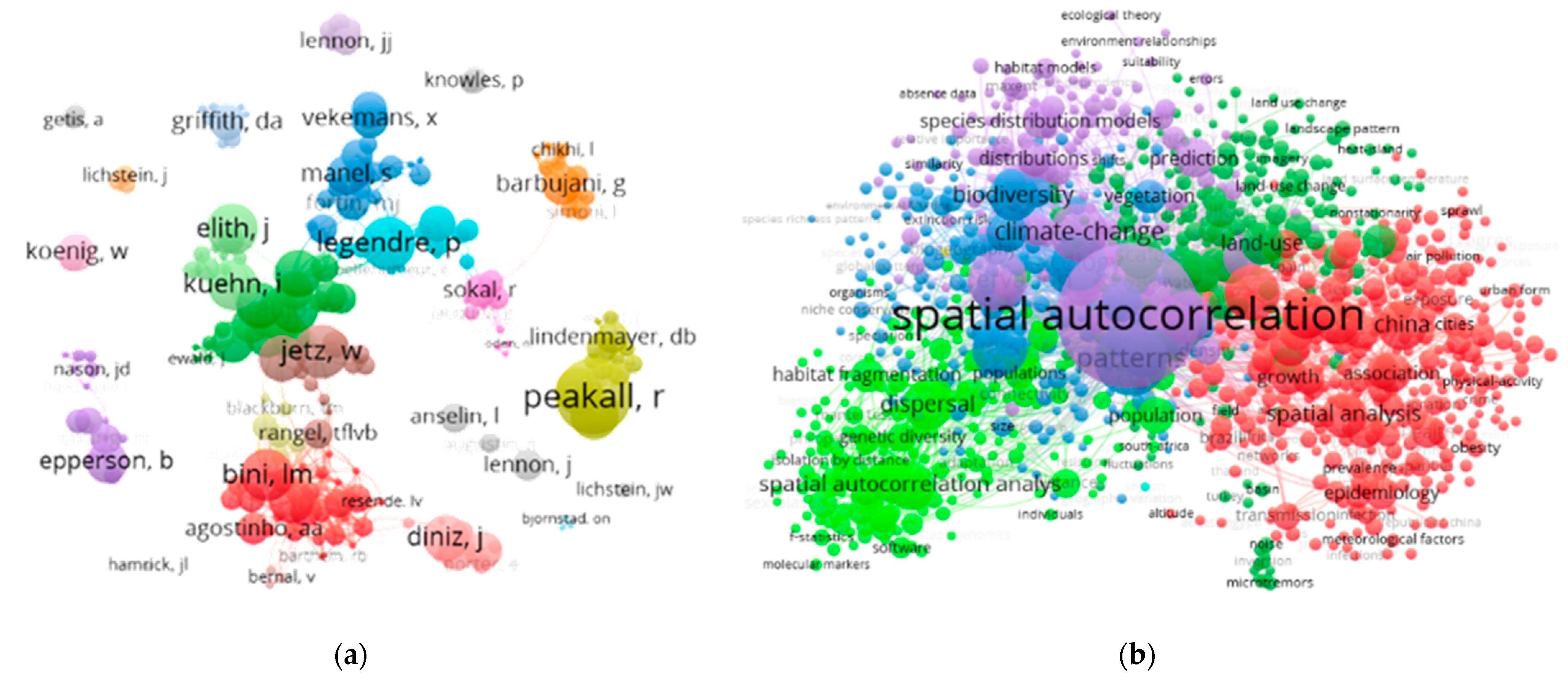
Figure 1. Web of Science (2012–2018) SA keyword cloud infographics (arbitrary group coloring visually differentiates among perceived SA research communities; node size reflects weighted normalized citation counts, which tend to highlight leading community scholars); compilation and portrayals by Drs. Kai Hu (Jiangnan University) and Qing Luo (Wuhan Institute of Technology). Left (a): authors. Right (b): concepts.
2. SA: An Important Geospatial Synoptic Statistic
Elementary descriptive statistics are important for quantitative analyses because they condense a numerical dataset’s information content into a few informative summary values about those data. Two vital descriptors are the mean and the variance because they respectively reveal a typical value and the spread of a dataset, even if the mean is a function of other variables when treated in a multivariate context. SA becomes a third crucial descriptor for georeferenced data—Goodchild [25] describes it as being endemic—because, in part, it exposes the presence of inflation in the variance, and, in part, because it represents redundant information that supplies the “essential economies that allow complex surfaces to be represented in manageable volumes” [25].
Couching this SA notion within a more technical statistical context, Legendre [28] emphasizes the commonly cited undermining by SA of the standard statistical analysis independent observations assumption, mentioning that it most often materializes in a geographic distribution as patches or gradients. Haining [27] highlights this SA non-independence feature as being instrumental to geography’s contribution to spatial statistics, commenting that SA relates to both scale and resolution of geographic data. Cliff and Ord [14] acknowledge that mis-specified regression models can create spurious residual SA, a theme discussed in detail by McMillen [29], and in terms of omitted variable beckoning by Griffith and Chun [31], can introduce omitted variable bias, especially in the presence of disregarded negative SA [32]. In these two latter multivariate contexts, a response variable’s mean varies, rather than being a constant (e.g., only an intercept term); SA contained in a response variable is a function of either that latent in related covariates, or spatial lag terms appearing in spatial autoregressive model specifications (e.g., conditional autoregressive (CAR), simultaneous autoregressive (SAR), and autoregressive response (AR) versions being the most popular) that attempt to usurp missing variable effects. Meanwhile, Goodchild [25] echoes the sentiment of the preceding paragraph, noting that SA is “… a monotonically decreasing function of distance [and hence] a fortunate characteristic of a wide range of spatially distributed phenomena.”
3. SA and Geographic Scale/Resolution
Legendre [28] addresses the geographic scale (i.e., geographic landscape size, relating to increasing domain sampling designs) issue, arguing that SA-related global patterns across a geographic landscape materializing as gradients arise from spatial (e.g., distance decay) processes or wide-ranging underlying common factors that elicit the formation of comparable outcomes in different regions and locations. Likewise, SA-related local patterns, which, landscape-wide, appear as disjoint patches separated by interstices, elicit the formation of numerous geographically small concentrations of outcomes at dispersed locations. Geographic scale provides the perspective that casts a clustering of similar values as being a gradient or patchiness. Pawley and McArdle [33] partner this scale issue with a recognition that the target of inference helps determine when SA presents data analysis complications or an opportunity to achieve additional effectiveness and/or robustness.
The geographic resolution (i.e., size of an areal unit polygon, relating to infill spatial sampling designs) issue involves some sort of data averaging within polygons: as polygons increase in size, more geographic averaging occurs, which has an accuracy highly correlated with any latent degree of positive SA. This averaging implies that, in practice, the SA measurements should change as resolution becomes coarser. Employing regular square quadrats, Chou [34] finds that SA measures increase in magnitude as resolution becomes finer, at a logarithmic rate; Zhang et al. [35] essentially corroborate this finding. Rodrigues and Tenedorio [36] report that the shape of irregular areal unit polygons also impacts SA measures, with aggregation of such nonuniform shapes varying in size not necessarily strictly rendering decreasing values with increasing coarseness. Di et al. [37] also detect an inverse relationship between resolution and SA measurement, while uncovering a tendency for SA quantifications to decrease in magnitude when irregular replace regular square shaped areal unit polygons. Describing this situation as the resolution sensitivity of SA, Mohan et al. [38] show that the aforementioned negative relationship is not necessarily a monotonically decreasing function—a finding similar to that by Rodrigues and Tenedorio [36]—devising a resolution correlogram tool based upon popular SA indices to adjust for this sensitivity.
The principal implication here for the metaphor explicated is that the sizes, shapes, and numbers of jigsaw puzzle pieces [39] affect the interface between a puzzle and SA addressed in the ensuing discussion. It also alludes to the issue of geographic scale and resolution. If a puzzle’s size is held constant, then increasing its number of pieces (all of which frequently are alike in total area) is equivalent to changing its geographic resolution. As geographic resolution increases, visual clues from puzzle pieces become more obscure; as geographic resolution decreases, clues from border buffer areas becomes more informative. Although artwork, piece size/shape, and color range can contribute to the degree of difficulty for solving a given puzzle, its number of pieces tends to be most strongly directly correlated with its degree of difficulty. As noted in the preceding paragraph, SA exhibits a similar type of tendency: it tends to increase in magnitude as resolution becomes finer, at a logarithmic rate.
References
- Salvati, L. Editorial: Introduction to a new open access journal by MDPI. Geographies 2020, 1, 1–2.
- Griffith, D. Spatial autocorrelation is everywhere. In Our Geographical Worlds: Celebrating Award-Winning Geography at the University of Toronto 1995 to 2018; Macijauskas, J., Ed.; Department of Geography and Planning & Association of Geography Alumni, University of Toronto: Toronto, ON, Canada, 2022; pp. 1–11.
- Tobler, W. A computer movie simulating urban growth in the Detroit region. Econ. Geogr. 1970, 46, 234–240.
- Williams, A. The Jigsaw Puzzle: Piecing Together a History; Berkley Books: New York, NY, USA, 2004.
- Monmonier, M. Air Apparent: How Meteorologists Learned to Map, Predict, and Dramatize Weather; University of Chicago Press: Chicago, IL, USA, 2000.
- Student. The elimination of spurious correlation due to position in time or space. Biometrika 1914, 10, 179–180.
- Yule, U. Why do we sometimes get nonsense-correlations between time series? A study in sampling and the nature of time series. J. R. Stat. Soc. 1926, 89, 1–69.
- Neprash, J. Some problems in the correlation of spatially distributed variables. Proc. Am. Stat. J. 1934, 29, 167–168.
- Stephan, F. Sampling errors and interpretations of social data ordered in time and space. Proc. Am. Stat. J. 1934, 29, 165–166.
- Fisher, R. The Design of Experiments; Oliver and Boyd: Edinburgh, UK, 1935.
- Yates, F. The comparative advantages of systematic and randomized arrangements in the design of agricultural and biological experiments. Biometrika 1938, 30, 444–466.
- Moran, P. Notes on continuous stochastic phenomena. Biometrika 1950, 37, 17–23.
- Geary, R. The contiguity ratio and statistical mapping. Inc. Stat. 1954, 5, 115–145.
- Cliff, A.; Ord, J. Spatial Autocorrelation; Pion: London, UK, 1973.
- Journel, A.; Huijbregts, C. Mining Geostatistics; Academic Press: New York, NY, USA, 1978.
- Paelinck, J.; Klaassen, L. Spatial Econometrics; Saxon House: Farnborough, UK, 1979.
- Anselin, L. Spatial Econometrics; Kluwer: Dordrecht, Germany, 1988.
- Cressie, N. Statistics for Spatial Data; Wiley: New York, NY, USA, 1991.
- Haining, R. Spatial Data Analysis in the Social and Environmental Sciences; Cambridge University Press: Cambridge, UK, 1996.
- Anselin, L. Local indicators of spatial association LISA. Geogr. Anal. 1995, 27, 93–115.
- Griffith, D. A family of correlated observations: From independent to strongly interrelated ones. Stats 2020, 3, 166–184.
- Goodchild, M. Spatial Autocorrelation; Concepts and Techniques in Modern Geography 47; Geo Books: Norwich, UK, 1986.
- Odland, J. Spatial Autocorrelation; SAGE: Thousand Oaks, CA, USA, 1988.
- Getis, A. A history of the concept of spatial autocorrelation: A geographer’s perspective. Geogr. Anal. 2008, 40, 297–309.
- Goodchild, M. What problem? Spatial autocorrelation and geographic information science. Geogr. Anal. 2009, 41, 411–417.
- Griffith, D. What is spatial autocorrelation? Reflections on the past 25 years of spatial statistics. L’Espace Géographique 1992, 21, 265–280.
- Haining, R. Spatial autocorrelation and the quantitative revolution. Geogr. Anal. 2009, 41, 364–374.
- Legendre, P. Spatial autocorrelation: Trouble or new paradigm? Ecology 1993, 74, 1659–1673.
- McMillen, D. Spatial autocorrelation or model misspecification? Int. Reg. Sci. Rev. 2003, 26, 208–217.
- Luo, Q.; Hu, K.; Liu, W.; Wu, H. Scientometric analysis for spatial autocorrelation-related research from 1991 to 2021. ISPRS Int. J. Geo-Inf. 2022, 11, 309.
- Griffith, D.; Chun, Y. Evaluating eigenvector spatial filter corrections for omitted georeferenced variables. Econometrics 2016, 4, 29.
- Griffith, D. Spatial autocorrelation mixtures in geospatial disease data: An important global epidemiologic/public health assessment ingredient? Trans. GIS 2023, 27, 730–751.
- Pawley, M.; McArdle, B. Spatial Autocorrelation: Bane or Bonus? bioRxiv. 2018. Available online: https://www.biorxiv.org/content/10.1101/385526v1.article-info (accessed on 24 August 2023).
- Chou, Y. Map resolution and spatial autocorrelation. Geogr. Anal. 1991, 23, 228–246.
- Zhang, B.; Xu, G.; Jiaoa, L.; Liua, J.; Donga, T.; Lia, Z.; Liu, X.; Liu, Y. The scale effects of the spatial autocorrelation measurement: Aggregation level and spatial resolution. Int. J. Geogr. Inf. Sci. 2019, 33, 945–966.
- Rodrigues, A.; Tenedorio, J. Sensitivity Analysis of Spatial Autocorrelation Using Distinct Geometrical Settings: Guidelines for the Urban Econometrician. In Computational Science and Its Applications—ICCSA 2014; Murgante, B., Murgante, B., Misra, S., Rocha, A., Torre, C., Rocha, J., Falcão, M., Taniar, D., Apduhan, B., Gervasi, O., Eds.; Part III, LNCS 8581; Springer: Cham, Switzerland, 2014; pp. 345–356.
- Di, W.; Qingbo, Z.; Zhongxin, C.; Jia, L. Spatial autocorrelation and its influencing factors of the sampling units in a spatial sampling scheme for crop acreage estimation. In Proceedings of the 6th International Conference on Agro-Geoinformatics, Fairfax, VA, USA, 7–10 August 2017; pp. 1–6.
- Mohan, P.; Zhou, X.; Shekhar, S. Quantifying resolution sensitivity of spatial autocorrelation: A resolution correlogram approach. In Geographic Information Science: GIScience 2012; Xiao, N., Kwan, M.-P., Goodchild, M., Shekhar, S., Eds.; Lecture Notes in Computer Science; Springer: Berlin/Heidelberg, Germany, 2012; Volume 7478, pp. 132–145.
- Armstrong, B. Jigsaw puzzle cutting styles: A new method of classification. In Game Researchers’ Notes; American Game Collectors Association: Dresher, PA, USA, 1997.
More
Information
Subjects:
Geography
Contributor
MDPI registered users' name will be linked to their SciProfiles pages. To register with us, please refer to https://encyclopedia.pub/register
:
View Times:
794
Revisions:
2 times
(View History)
Update Date:
07 Oct 2023
Table of Contents


Notice
You are not a member of the advisory board for this topic. If you want to update advisory board member profile, please contact office@encyclopedia.pub.
OK
Confirm
Only members of the Encyclopedia advisory board for this topic are allowed to note entries. Would you like to become an advisory board member of the Encyclopedia?
Yes
No
${ textCharacter }/${ maxCharacter }
Submit
Cancel
Back
Comments
${ item }
|
${ item.createdUser.fullName }
${ item.createdAt }
${ item.vote }
${ item.reply }
Delete
${ reply.createdUser.fullName }
${ reply.createdAt }
${ reply.vote }
Delete
There is no reply to this comment~
${ item.replyTextCharacter }/${ item.replyMaxCharacter }
Submit
Cancel
More
No more~
There is no comment~
${ textCharacter }/${ maxCharacter }
Submit
Cancel
${ selectedItem.replyTextCharacter }/${ selectedItem.replyMaxCharacter }
Submit
Cancel
Confirm
Are you sure to Delete?
Yes
No