In the research field of simulation-based engineering science, there are three categories of computational modelling methods, in terms of how to implement spatial discretisation. They include the Eulerian method, the Lagrangian method and the hybrid method
[1]. In the Eulerian method, the computational grid does not move with the fluid flow or material deformation, while there is advection of mass between the target material and the computational grid. In the Lagrangian method, however, the computational grid moves with the flowing/deforming target material. The hybrid method uses some techniques to combine the Largangian approach with the Eulerian approach. The successful employment of an arbitrary Lagrangian–Eulerian (ALE) method in the finite element (FE) analysis software ABAQUS is a good example of the application of hybrid methods in computational modelling. The ALE adaptive meshing makes the FE computational grid “move independently of the target material”, to “maintain a high-quality mesh throughout an analysis”
[2]. Regardless of what method is used to implement the spatial discretisation, the target material is assumed to be either continuous (e.g., single material/phase problems) or piecewise continuous (e.g., multi-material or multiphase problems) in the computational modelling of continuum mechanics problems. For example, in the FE modelling of solid mechanics problems, a constitutive equation, in conjunction with related boundary conditions and material properties, is solved on an FE grid, to computationally solve the boundary-value problems of solid mechanics problem. Regarding the computational fluid dynamics (CFD) modelling of single-phase incompressible Newtonian fluid flow and heat transfer problems using the finite volume method
[3], it is typical that the Navier–Stokes equations are solved on an Eulerian or Lagrangian finite volume grid. Regarding the level set method for multiphase problems, the propagation/variation of the inter-phase interface is implicitly captured by solving the level set equation on a computationally grid
[4]. In the afore three examples, regardless of whether the target material is uniform (such as in the FE analysis of isotropic linear elastic materials and the CFD modelling of single-phase materials) or non-uniform (e.g., in the level set modelling of multiphase problems), the target material is always assumed to be continuous or piecewise continuous.
The benefit of treating the target material as a mathematically continuous (or piecewise continuous) medium in the computational modelling is very obvious. Firstly, it directly reflects the fundamental concept of continuum mechanics, which study the macroscopic behaviour of materials by using a continuous outlook (i.e., treating the target material as a continuous mass)
[5]. Secondly, related computational modelling is normally computationally efficient. In the continuum mechanics, the particulate nature of target materials (such as material microstructure, defects, inter-atomic interactions, etc.) are not explicitly considered. The influence of such particulate nature (or properties) of the target material is normally implicitly and indirectly taken into account in the continuum mechanics by employing related macroscopic properties of the target material (such as elasticity and plasticity of solid materials, the viscosity and density of fluids, etc.) in the continuum mechanics. Related computational methods are applicable to the modelling of an appreciable volume of material (e.g., up to the volume of an entire engineering component) during a process of appreciable length (e.g., comparable to an entire engineering process).
All engineering materials consist of discrete entities (such as atoms, molecules, grains, defects, etc.). When a “discrete outlook” concept is employed, it regards the target material as a population of individual material points (or particles) that interacts with one another at very short distances
[5]. Such a particulate approach studies the properties of the particulates and the interaction between the particulates. The particulates can be, as examples, atoms, molecules or any other microscopic particulates. Such an approach relates to discrete mechanics
[6]. Regarding the computational modelling of materials using the concept of discrete mechanics, molecular dynamics (MD) is a good example. In MD, the target material is assumed to consist of a population of individual but interacting atoms
[7]. The interaction can be mathematically formulated by using a potential function. MD implements classical mechanics to study the classical motion of many-body systems. It has been successfully employed to computationally predict, for example, the solidification of metals at the nanoscale
[8], the welding of thermosetting polymers
[9], the roll casting of Cu/Al clad plates
[10] and extensive additive manufacturing
[11].
On the one hand, the modelling methods using the particulate approach can directly reflect the microscopic processes and phenomena of materials (e.g., the motion and interactions of atoms of the target material). On the other hand, such a modelling method is very computationally costly and is normally only applicable to a very small volume of material. For example, as was reviewed in
[12], there are normally a limited number of atoms in an MD simulation domain and the time window is typically on the order of magnitude of hundreds of picoseconds. It is often applied regarding the finite-size effects of such an incredibly small simulation domain (on the nanoscale)
[13]. Due to such a limited length of time that can be considered in MD simulations, normally only very extreme levels of cooling rate (e.g., on the order of 10
5 K/s
[13]) can be employed in the modelling of a material during cooling.
It is clear that the modelling methods based on the “continuous outlook” concept suit applications in a large volume of material that can provide the macroscopic properties of the target material or process. The modelling methods based on the “discrete outlook” concept suit applications where the particular delicate interaction between particulates of the material is the main interest of research. In the application of computational modelling in science and engineering, there is a type of scenario where some delicate processes of a macroscopic system need to be computationally formulated and predicted. One good example of such a scenario is predicting the flow of fluid in porous media. If one only cares about the overall macroscopic properties of the flow, such as the overall static pressure loss of fluid across the porous media, one can very easily use the common Darcy’s law (or its variants) in a conventional CFD modelling based on the finite volume method
[14] to get the job done. Darcy’s law assumes the porous media is a continuous uniform permeable material, i.e., a “continuous outlook”. Rather than considering the individual pores, Darcy’s law uses a loss coefficient to characterise the macroscopic properties of the porous media regarding the fluid pressure loss. However, if one cares about the pore-scale characteristics of a complex flow problem (such as multiphase flow in heterogeneous porous media)
[15][16], special care must be taken. For example, if the modelling needs to be applied to the flow problem in an appreciable volume of porous media, the “discrete outlook” that considers the actual atoms is not applicable because its computational cost is unaffordable. Some other good examples of such special scenario include high speed impact
[17], immiscible multiphase flow
[18], fluid–structure interaction
[19] and flow/heat transfer involving moving boundaries
[20]. All these problems in this special scenario either have complex (or moving) interfaces or involve significant and complex (as well as delicate) interface topological changes.
2. Lattice Boltzmann Method
Lattice Boltzmann method (LBM) is a type of lattice-based pseudo-particle method. It combines the concept of material pseudo-particles (which was firstly used in the Lattice Gas Automata method) with the kinetic equations of related processes (i.e., the Boltzmann Equation)
[21]. When the LBM is employed to formulate the fluid dynamics problems, it satisfies the Navier–Stokes equation on one hand, but does not explicitly solve the Navier–Stokes equation on the other hand. In the LBM, the interaction between material elements is reflected in the concept of collisions of pseudo-particles, which is mathematically formulated by using the kinetics of the probability distribution function (i.e., the Boltzmann Equation):
where
𝑓 is the probability distribution function,
𝜉 is the microscopic velocity in a direction,
t is time and
F is the external body force.
Ω formulates the collisions between pseudo-particles, which are affected by how the material elements interact with one another as well as the material properties. For example, for fluid dynamics problem,
Ω relates to the viscosity, speed of sound, temperature, density and molar mass of the target fluids.
By using the BGK model in conjunction with the single relaxation time approach, the discretized Boltzman equation can be formulated as
[22]
where
𝑒𝑖 is the velocity in the
i direction of the computational grid,
𝜏 is the dimensionless relaxation time and
𝑓𝑖(𝑥,𝑡)𝑒𝑞 is the Maxwell–Boltzmann equilibrium probability distribution function, which only depends on the material properties.
𝐹𝑖(𝑥,𝑡) accounts for the body force as well as the forces due to the interactions between material elements. The probability distribution function can be used to derive the macroscopic properties (such as density and momentum density) of the target material for single-phase or multiphase problems:
where
u is the actual macroscopic velocity of a material element and
𝑒𝑖 is the discrete probable velocity of the material element in the probable direction
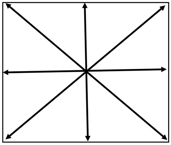
i. The LBM is normally implemented based on a structured computational grid. For either single-phase problems or multiphase problems, normally the computational grid is static and does not move/deform with fluid flow or solid deformation. It is the temporal and spatial variation in the probability distribution function that reflects the processes of, for example, fluid flow and solid deformation. Therefore, the LBM is normally a type of Eulerian method. The type of LBM computational grid is normally categorised by using codes such as DxQy, where
x represents the number of dimensions and
y represents the number of directions in which the information of a pseudo-particle can propagate. For example,
Figure 1 displays the D2Q9 computational grid that is widely employed in 2D LBM modelling. There are many different types of computational grids that can be employed in LBM modelling. The choice of computational grid depends on information such as the number of dimensions of the target problem, the expected level of accuracy, the affordable computational cost, etc. It is worth noting that different weighting coefficients may apply to different directions in an LBM computational grid. When solving the Boltzmann equation, there are two steps: the Collision Step and the Streaming Step. The Collision Step corresponds to the process of the particle of interest colliding with the neighbouring particles, which reflects the relaxation of probability distribution function
f towards the local equilibrium. The Streaming Step reflects the process of information propagation from the particle of interest towards the particles nearby. Related details of the mathematical background of the LBM method can be seen in
[21].
When the probability distribution function
f only represents the likelihood of a material element having a particular velocity in a particular direction at a particular location, the corresponding LBM can be employed in the CFD modelling of fluid flow problems
[23][24]. When the probability distribution functions can characterise not only velocity but also temperature (or thermal energy) of the fluid at the nodes of the computational grid, the corresponding LBM can be employed in the modelling of fluid flow in conjunction with heat transfer. For example, in the LBM modelling performed by Semma et al.
[25], a double distribution function method was used, which used one probability distribution function to formulate the flow problems and a different probability distribution function to separately formulate the heat transfer problems. If a third probability distribution function of the material solute concentration can be considered in the LBM
[26], the process of fluid flow in conjunction with heat transfer and solute transport can be simulated.
3. LBM and Enthalpy Method
Regarding the phase transformation between the liquid and solid phases during solidification or remelting, a particular model of phase transformation is needed to formulate this, as the LBM itself is incapable. An approach similar to the enthalpy formulation of phase transformation was employed by Semma et al.
[25] in the computational modelling for melting/solidification problems of pure gallium in a square cavity under the influence of natural convection, which was supported by related verification and validation. In the Enthalpy Method of phase transformation, the evolution of material enthalpy follows the below partial differential equation
[27]:
where
H is enthalpy,
T is temperature,
u is fluid macroscopic velocity,
𝑘 is thermal conductivity and
𝐶𝑝 is specific heat capacity. The enthalpy can be calculated as the sum of the sensible enthalpy and latent heat of fusion. The volume fraction of liquid phase is assumed to be a linear function between the enthalpy of the material at the liquidus temperature and the enthalpy at the solidus temperature. The energy equation is not explicitly solved in the LBM modelling. Again, a collision-streaming approach is used to update the probability distribution function in relation to enthalpy:
where
𝑔𝑖 is the probability distribution density of enthalpy in the
i direction of the computational grid,
𝑔𝑖(𝑥,𝑡)𝑒𝑞 is the Maxwell–Boltzmann equilibrium probability distribution function relating to the enthalpy and
𝐻(𝑥,𝑡)=∑𝑖𝑔𝑖(𝑥,𝑡). Depending on the specific assumptions of the problems, either single relaxation time scheme or multiple relaxation time scheme can be employed in the solution processes.
4. LBM and Cellular Automata Method
The LBM model employing the enthalpy formulation mainly computationally formulates the process of phase transformation in the perspective of change of enthalpy of the target materials. If the specific mechanisms and mathematical formulas of solute partition in conjunction with solute diffusion/convection are well understood, the process of phase transformation (solidification or remelting) can be assumed to be driven by the difference between the local interface equilibrium composition and the local actual liquid composition of material—if the liquid phase and solid phase can be assumed to be locally in equilibrium at the interface. For example, in the modelling of the dendritic growth process during natural and forced convection
[26][28], it was assumed that the interface equilibrium composition of the liquid phase was
where
𝑇∗𝑙 is the interface temperature,
𝑇𝑒𝑞𝑙 is the equilibrium liquidus temperature at the initial composition
𝐶0,
𝐶∗𝑙 is the interface equilibrium solute concentration of the liquid phase,
𝜀 is the degree of anisotropy of the surface tension,
m is he liquidus slope of the phase diagram,
Γ is the Gibbs–Thomson coefficient,
K is the curvature of the solid–liquid interface,
𝜃 is the growth angle between the normal to the interface and a reference direction and
𝜃0 is the angle of the preferential growth direction with respect to the reference direction.
The change in solid fraction of the target material can be formulated as a function of the interface equilibrium composition of the liquid phase and the actual composition of the liquid phase:
where
k is the solute partition coefficient
𝑘=𝐶𝑠/𝐶𝑙,
𝐶𝑠 and
𝐶𝑙 are the solute concentration in the solid phase and liquid phase and
𝜙𝑠 is the solid fraction. The release of solute into the liquid phase and the release of latent heat can be formulated as
where
𝐶𝑝 is the specific heat capacity,
𝜙𝑠 is the solid fraction,
T is temperature and
L is the latent heat of fusion. The values of
Δ𝐶𝑙 and
ΔT, in conjunction with fluid velocity, can be used to update the probability distribution functions of fluid flow, heat transfer and solute transport. This type of computational modelling for the microstructural evolution during phase transformation as well as its variants (such as
[29][30]) are called Cellular Automata (CA) methods. In a typical CA model for phase transformation, the interface between different phases is assumed to have the thickness of one computational cell. Such an assumption provides the convenience of developing related computational models and has nothing to do with the actual thickness of the interface. Regarding the transformation between the solid phase and liquid phase, each computational cell can only be in one of the three discrete states: liquid state, solid state and interface state. Only in the interface cells can the solid fraction be less than one and greater than zero. The value of
Δ𝜙𝑠 can be used to characterise the process of phase transformation happening in each interface cell. The propagation of the interface cells explicitly reflects the process of microstructural evolution during solidification. That is to say that there is a sharp jump between two different phases across the interface.
5. LBM and the Phase Field Method
The phase field (PF) method is a diffusive interface method, which has very smooth and continuous variation across an interface between, for example, the liquid phase and the solid phase. In the LBM+CA model of phase transformation, as used in
[26][28], the process of phase transformation is solely determined by the conserved field variable—solute concentration of alloy. In the PF model of phase transformation, the phase transformation is characterised by a non-conserved field variable order parameter, which smoothly varies between 1 (solid phase) and −1 (liquid phase) regarding the phase transformation between the liquid phase and solid phase. In the LBM+PF modelling of Rátkai et al.
[31] and Zhan et al.
[32], an Allen–Cahn equation governing the order parameters in conjunction with a Cahn–Hilliard equation governing the solute partition and transport was solved. The LBM+PF modelling was used to predict the sedimentation of equiaxed dendrites as well as the influence of natural convection on them in microgravity
[31], along with the influence of forced thermosolutal convection on the growth of equiaxed dendrites
[32].
6. Application of LBM Modelling
The LBM method has been widely employed in the computational modelling of a variety of material processing and manufacturing processes, such as casting, welding and additive manufacturing (AM).
By using the large eddy simulation (LES) model to treat the turbulence, the LBM was employed in computational modelling to predict the fluid vortex and turbulence inside the submerged entry nozzle as well as near the mould wall of a continuous casting process
[33]. The free surface flow problem of molten metal was treated as a melt–air two-phase flow problem, and the density of air was assumed to be zero. The collision-streaming approach was used to update the volume fraction of liquid for all computational cells, implementing the propagation of the melt–air interface during the melt flow during the continuous casting.
Regarding the modelling for welding, the LBM was integrated with the enthalpy method to computationally predict the remelting and, particularly, the Marangoni flow during the plasma arc welding of steels
[34]. The LBM+CA method was employed to computationally predict the evolution of solidification structure during the arc welding of Inconel 601H
[35].
Regarding the application of the LBM in the computational modelling of additive manufacturing (AM) processes, Korner and co-authors have made extensive publications in this field. By using the LBM method, they computationally predicted how the evaporation process may affect the heat and mass transfer of the melt pool as well as the influence of the recoil pressure on the geometry of the melt pool during the electron beam powder bed fusion (EB-PBF) AM of a Ti alloy
[36]. Practically, their LBM modelling was implemented to predict the process window of EB-PBF AM regarding, as examples, how the powder bulk density
[37] or hatching process strategies
[38] may affect the result of the EB-PBF AM of Ti alloys. By using the LBM+CA method
[39], the evolution of the solidification structure of IN718 during the EB-PBF AM was computationally predicted. In addition to completing some model validation, the influences of the hatching strategy on solidification structure as well as the formation of partially molten powder particles were predicted using the modelling.
By integrating the LBM with the enthalpy method
[40], Chen et al. computationally predicted (in 3D) the geometry of the consolidated Ti-6Al-4V tracks manufactured using EB-PBF AM, as well as the influence of process parameters.
While having extensive advantages, the LBM has some limitations too. For example, by employing the Chapman–Enskog analysis, the LBM can be automatically reduced to the continuity equation and momentum equation of incompressible flow problems in the limit of small Knudsen number and low Mach number
[41]. If the LBM needs to be employed in the modelling of compressible flow problems at high Mach numbers, special care must be taken. In the computational modelling of immiscible multi-fluid flow using LBM, spurious currents may exist in the modelling results if the density ratio between two fluids is high. Such spurious currents may increase with the density ratio, contributing to the numerical instability of the LBM
[21]. Special techniques need to be developed in order to use LBM in the modelling of multi-fluid problems that have relatively large density ratios. When trying to increase the stability of LBM models, different collision models have been developed. The physical interpretations of the collision models and why they may influence the model stability are still insufficient
[42]. The LBM may also have some difficulties in the computational modelling of micro-flow problems.
 +1 credit