Probabilistic Decline Curve Analysis Approaches

Version	Summary	Created by	Modification	Content Size	Created at	Operation
1		Taha Adbelhamid Yehia	--	3341	2023-06-09 17:59:30	\|
2	reference editing	Taha Adbelhamid Yehia	Meta information modification	3341	2023-06-09 18:46:24	\| \|
3	layout	Sirius Huang	Meta information modification	3341	2023-06-12 04:22:16	\|

This entry is adapted from the peer-reviewed paper 10.3390/en16104117

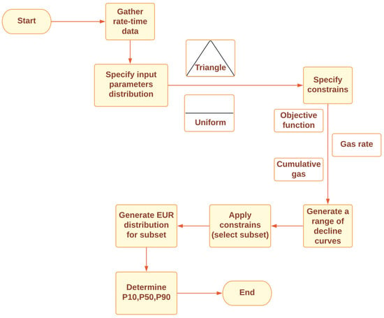
The decline curve analysis (DCA) technique is the simplest, fastest, least computationally demanding, and least data-required reservoir forecasting method. Assuming that the decline rate of the initial production data will continue in the future, the estimated ultimate recovery (EUR) can be determined at the end of the well/reservoir lifetime based on the declining mode. Many empirical DCA models have been developed to match different types of reservoirs as the decline rate varies from one well/reservoir to another. In addition to the uncertainties related to each DCA model’s performance, structure, and reliability, any of them can be used to estimate one deterministic value of the EUR, which, therefore, might be misleading with a bias of over- and/or under-estimation. To reduce the uncertainties related to the DCA, the EUR could be assumed to be within a certain range, with different levels of confidence. Probabilistic decline curve analysis (pDCA) is the method used to generate these confidence intervals (CIs), and many pDCA approaches have been introduced to reduce the uncertainties that come with the deterministic DCA.

probabilistic decline curve analysis estimated ultimate recovery confidence intervals data sampling

1. Introduction

Different decline curve analysis (DCA) models have been recently developed and used, especially for unconventional shale reservoirs ^[1]^[2]^[3]. There are several uncertainties in estimating the ultimate recovery(EUR) using one or more DCA models ^[4]^[5]^[6]. To assess the uncertainty in reserve estimations based on DCA, analysts are increasingly using probabilistic techniques because the results are based on a statistical study of historical data, which frequently have a lot of noise ^[7]^[8]. When production profiles show an unknown behavior at a late time during an evaluation of the reservoirs, uncertainty analysis is extremely important. Hence, it is essential to predict production using a probabilistic methodology ^[9].

The challenge in estimating probabilistic reserves using DCA is not only in determining how to identify the probabilistic features of complicated production data sets but also in determining which approach (i.e., set of steps) should be followed to improve the reliability of the uncertainty quantification and forecasting of the reserve with a higher level of confidence.

2. pDCA Approaches

pDCA is one of the analysis tools used to quantify and reduce uncertainties. However, the basis of analysis also carries uncertainties. Those uncertainties are mainly related to the assumptions of the probability distributions of the parameters, the sampling techniques, and the computational time. All of these reasons and more have led to the development of several pDCA approaches to make it more effective in predicting the production and narrowing the bounds of P₁₀, P₅₀, and P₉₀.

As mentioned earlier, pDCA is based on providing probability distributions of the parameters of a selected DCA model(s). Here, some questions should be asked, such as: Which model or a combination of models should be used? What was the used sampling technique? What is the type of probability distribution to be assumed that the model’s parameter/s are following? What is/are the parameter(s) to be probability distributed? The different answers to and preferences of these questions have led to the development of many pDCA approaches.

2.1. Jochen’s Approach (1996) ^[10]

Jochen and Spivey introduced the bootstrap sampling technique, which is related to DCA models ^[10]. The motivation behind this work was the reason for building the probability levels of interest (i.e., P₁₀, P₅₀, and P₉₀) based on the deterministic results. The simple assumption that the model’s parameters are following a certain distribution is not efficient and easily could be wrong. The authors showed that the unreliability related to such pDCA approaches was due to the use of the same original data to create a probability distribution of the estimator’s (i.e., the selected DCA model’s) parameters. Therefore, the bootstrap technique was used to resample the original data several times and the MC simulation was used to create the probability distribution and estimate P₁₀, P₅₀, and P₉₀. Moreover, they proved that if the number of iterations is larger than 100, the trend will be the same.

Although this method does not require previous knowledge about the prior distributions of the parameters, it assumes that there is no relation between the original data (i.e., independent) and it follows the same distribution, which is wrong as the production data points are, somehow, correlated, and therefore, they are considered a time-series-data structure. Moreover, creating several synthetic data sets from the original production data make this approach computationally intensive, as was reported in their studies.

2.2. Cheng’s Approach (2010) ^[11]

To preserve the data structure, two more steps were added to mitigate the assumptions of the Jochen approach, where Cheng et al. introduced what they called the modified bootstrap method (MBM) ^[11]. The first step was to perform a nonlinear regression with a hyperbolic or exponential model to fit the production data, and the second step was to use a block resampling of the autocorrelated residuals obtained from the fitted DCA model (Arps, in this case) to the actual data. In the end, the regressed production data are then sampled several times to create synthetic data sets and the accuracy of MBM is dependent on the block size. Table 1 states the differences between Jochen’s and Cheng’s approaches while Figure 1 shows Cheng’s approach modifications to the bootstrap sequence.

Figure 1. A scheme that shows the modifications to Jochen’s approach by Cheng.

Table 1. The differences between Jochen’s and Cheng’s approaches.

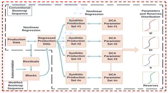
Jochen’s Approach	Cheng’s Approach
Uses bootstrap as a sampling technique
Uses Arps’ models as the DCA model
Assumes no correlation between the data points	Assumes a time-series-data structure
Resampled the original data	Resampled the fitted data obtained from a DCA model (Arps)
Random samples from the original data are generated	Samples are generated based on autocorrelated residual blocks

In testing Cheng’s approach on 100 oil and gas wells, the coverage range (CR) was improved to 83% compared to the original approach by Jochen (34%). It was suggested that reusing this approach after fitting the recent production history will lead to improving the CR of future production within an 80% CI, as shown in Figure 2. This is called a backward scenario. Conventionally, when all of the production history is used for regression, the actual performance becomes outside of the 80% CI. On the other hand, when only the recent production history is used for regression, the actual performance is within the 80% CI.

Figure 2. The “backward scenario”.

Although the MBM has proven to be well-calibrated in unconventional reservoirs ^[12], it could be inferred that the efficiency of the forecasting decreases for the far future because the interval width becomes wider.

2.3. Minin’s Approach (2011) ^[13]

The Arps relationship was utilized to analyze 150 horizontal and hydraulically fractured shale gas wells using the pDCA approach and the conventional MC sampling method ^[13]. A probability distribution was created for the initial decline rate (D_i), decline exponent (b), initial flow rate (q_i), and the initial flow rate divided by the lateral length of the wells (q_i, n). Additionally, they estimated the cumulative distribution functions (CDFs) for each parameter four times (i.e., one CDF after each year of production). They concluded that with time, the b-exponent tended to decrease and stabilize, and D_i tended to increase and stabilize. This is because the flow regime is shifted with time from transient to BDF. Moreover, an incensement of the q_i could be related to the incensement of the lateral horizontal length in the case of drilling a new development well. In addition, there could be a negative correlation between q_i and the horizontal length after reaching a certain length.

The novelty of this work was the conducted pDCA to quantify the uncertainty, and to characterize the flow regime changes with time. It was also used to recommend a drilling design in the case of further development of wells.

2.4. Gong’s Approach (2011) ^[12]

DCA based on Bayesian statistics was first introduced by Gong ^[12]. The MCMC sampling technique based on the MH algorithm was used to obtain the posterior distribution of the Arps parameters.

The approach was tested based on 197 shale gas wells. There were two main advantages were related to this work: (1) compared to the MBM method, this approach was 10 times faster, and (2) unlike using the MBM method, the CI did not diverge too much in forecasting the far future. Figure 3 shows a comparison between Gong’s approach and the MBM approach when both approaches are applied to the same dataset.

Figure 3. A comparison between Gong’s approach and the MBM approach.

2.5. Brito’s Approach (2012) ^[14]

Working on multiple wells rather than a single well, Brito introduced an approach based on a normalized rate called production decline envelopes (PDE) ^[14]. This approach allowed for analyzing multiple wells and creating decline bands that could be used as the pDCA. This approach can be summarized in three steps, as shown in Figure 4.

Figure 4. Summary of Brito’s approach.

The maximum, average, and minimum decline curves can be seen as P₁₀, P₅₀, and P₉₀. The probability distribution is conducted to the initial flow rate and not to the selected DCA model parameters.

2.6. Gonzalez’s Approach (2012) ^[9]

Following the same steps proposed by Gong et al. (i.e., using the MCMC sampling technique and even the same data), Gonzalez et al. extended this work to be combined with more than one DCA model ^[9]^[15]. They used the Arps, modified Arps, Duong’s, PLE, and SEPD models with the MCMC sampling technique. They denoted that P₅₀ using Arps was the best amongst all of them, with the exception of the short production data, while PLE came second and performed well using the short production data. Overall, the estimated P₅₀ from any model was more reliable than each single deterministic reserve value. This work suggested that many DCA models can be combined with the MCMC technique. Comparing all of them can help in minimizing uncertainty about forecasting.

2.7. Fanchi’s Approach (2013) ^[16]

Fanchi introduced a simple approach to conduct a pDCA-based approach on any selected deterministic model ^[16]. Working on 110 shale gas wells from different fields and using the Arps and SEPD models, the authors proposed the steps of the approach shown in Figure 5. The MC simulation sampling technique was used to create a probability distribution of the chosen model’s parameters through 1000 iterations after selecting a certain probability distribution for them.

Figure 5. Summary of Franchi’s approach.

It should be pointed out that the study did not compare the results of the two proposed pDCA studies, and it did not present the coverage range of both of them. Therefore, it could not be considered a comparative analysis.

2.8. Kim’s Approach (2014) ^[17]

Appling both approaches introduced by Brito and Fanchi, but with small differences, Kim used the MC simulation sampling technique with 5000 iterations and a triangle probability distribution for a single well analysis based on the Arps and SEPD models (similar to Fanchi). Moreover, the PDE was applied for multiple-wells analysis, similar to Brito’s approach ^[17]. Compared to the previous works of Brito and Fanchi, Kim’s work introduced nothing new, but it used a triangle probability distribution instead of the uniform distribution followed by Fanchi. In addition, Kim performed 5000 iterations while Fanchi performed 1000 iterations.

2.9. Zhukovsky Approach (2016) ^[18]

Zhukovsky et al. worked on more than 200 shale oil wells ^[18]. The EUR was estimated using the EEDCA model. The authors used the MCMC simulation as the sampling technique with 100,000 iterations to estimate the posterior probability distribution of the EUR using Matlab software. Calculating P₁₀, P₅₀, and P₉₀ from the CDF, they found that the coverage rate of the 80% CI was 78.4% of the used DCA models, which was a good result. However, many wells showed high average relative errors and average absolute errors related to the actual EUR. They assigned these errors to the low quality of the data collected and being tested and not to the approach itself. Even if the resampling algorithms and different approaches could reduce some of these errors, the heavy noise and fluctuating data could lead to unreliable estimations.

2.10. Paryani’s Approach (2017) ^[19]

Paryani et al. introduced their approach by combining the Arp and logistic growth (LGM) models in a probability study ^[19]^[20]. It was based on using the ABC sampling technique to approximate the complicated likelihood function of the model’s parameters by 1000 iterations. The approach was tested based on 121 oil and gas shale wells from two different fields. They denoted that their approach was much faster and could be combined with other deterministic DCA models. They indicated that LGM was much better than the Arps model and provided better CRs. They also compared their approach with Gong’s approach, as shown in Figure 6. Based on this comparison, although the two approaches bounded the production history from P₁₀ to P₉₀, Paryani’s approach had narrower intervals, which indicated low uncertainty.

Figure 6. A comparison between Paryani’s and Gong’s approaches.

2.11. Jimenez’s Approach (2017) ^[21]

Working on tight gas reservoirs, Jiménez introduced an approach to estimate the reserves based on a probability study ^[21]. In this work, they started with a parametric study on the Arps model’s parameters D_i and b to determine which parameter affected the reserve estimation more than the other. They denoted that the b parameter had a greater effect than the D_i parameter. This was known before this work as the b exponent is the controller of the curvature degree. Therefore, it affects the EUR value more than the D_i parameter does.

Applying different DCA models (hyperbolic Arps, SEPD, PLE, and LGM), the authors determined the EUR from each model. They proposed that SEPD was the conservative model among them. Therefore, they conducted a probability study to calculate P₁₀, P₅₀, and P₉₀ based on the MC simulation sampling technique and Chi-square distribution of the model parameters.

2.12. Joshi’s Approach (2018) ^[22]

Joshi used a time series analysis technique and a frequentist statistical analysis to quantify uncertainty ^[22]. The LGM and SEPD models were used to test their approach on 100 shale gas wells. Based on de-trending (i.e., subtracting the deterministic trend of the model from the actual data), the time series autoregressive integrated moving average (ARIMA) model was integrated with the LGM and SEPD models to generate the CIs (i.e., P₁₀, P₅₀, and P₉₀) around the production forecast.

It could be inferred that by increasing the available production data for fitting, the 80% CI became narrower (i.e., the uncertainty decreased), as shown in Figure 7.

Figure 7. Results of Joshi’s approach when increasing the production data being fitted from (a–c).

Additionally, the authors also compared their approach with Gong’s approach, and they denoted that Gong’s approach was much more reliable as it had narrower CIs, as shown in Figure 8 ^[12]. The comparison could be considered as evidence of the effectiveness of the pDCA approach based on Bayesian analysis compared to the pDCA approach based on frequentist analysis.

Figure 8. A comparison between Gong’s and Joshi’s approaches.

2.13. Hong’s Approach (2019) ^[23]

Hong worked on nearly 69 unconventional oil wells from two different fields ^[23]. Four DCA models—Arps, SEPD, LGM, and Pan—were used. Using MATLAB software (MathWorks 2017a), they fitted each model 10 times using the cross-validation technique instead of the least squares estimation, which is commonly used in non-linear regression. This technique helped in improving the curve-fitting. The motivation behind this work was to determine which DCA model had the highest potential to perform pDCA among the other models. After choosing the prospective DCA model, the MC simulation sampling technique was used to generate a uniform distribution of the model’s parameters.

The authors concluded that the goodness of fitting was not a condition for the best model, but the best model was that one able to represent the actual flow behaviors. They also denoted that a large production history may not reduce the model’s uncertainty. Finally, and based on their work, Arps and LGM became more optimistic in estimating the reserve compared to the SEPD and Pan models. They did not indicate the number of iterations used to generate the uniform distribution or the computational time, which would have been important for evaluating their approach compared to other approaches.

2.14. Fanchi’s New Approach (2020) ^[24]

Fanchi introduced his pDCA approach after working on 15 shale oil wells in two different fields ^[24]. Using the MC simulation sampling technique, he created a uniform probability distribution of the used DCA models (Arps and SEPD) with 1000 iterations. The P₁₀, P₅₀, and P₉₀ were also estimated for both models. The study did not compare the results of the two proposed pDCA studies and denoted nothing about each study’s coverage. Therefore, it could not be considered a comparative analysis. The difference between this work and his previous work is that the domain of this study was shale oil while that of the previous work was shale gas.

2.15. Korde’s Approach (2021) ^[25]

Korde et al. worked on 74 conventional and unconventional wells (51 gas wells and 23 oil wells) to introduce their approach ^[25]. They used five DCA models (Arps, PLE, Duong, SEPD, and LGM). They assessed each DCA model based on three Bayesian sampling techniques (Gibbs, MH, and ABC). The probability distribution used was the maximum likelihood distribution. They introduced two ways to conduct the pDCA. The first was to choose one DCA model and evaluate the performance of the sampling techniques. They found that LGM performed well with all the sampling techniques except for MH. The second was to choose one sampling technique and evaluate the performance of all the DCA models. They found that the Gibbs algorithm performed well with all the DCA models except the Arps model. The computational time for each pDCA was between 2 and 25 s.

Figure 9 shows the different Bayesian sampling algorithms used in conjunction with the Arps model. It is easy to see how the interval width (IW) was the largest with the Gibbs algorithm and the lowest with the ABC algorithm. The author suggested that by preprocessing the data and reducing the noise, the IW was improved and the prediction errors were reduced.

Figure 9. The different Bayesian sampling algorithms that were used in conjunction with the Arps model: (a) MH algorithm, (b) Gibbs algorithm, and (c) ABC algorithm.

The authors also concluded that, adding more production data to the pDCA model improved its results. Therefore, conducting more than pDCA helped to assure the results of the EUR.

The major differences between the aforementioned pDCA approaches are clearly stated and summarized in Table 2. The sampling techniques, the study domain, the selected models, and the used probability distributions are categorized and compared.

Table 2. Summary of the pDCA approaches ^[26].

pDCA Model	Probabilistic Technique	Sampling Technique(s)	No. of Integrations	Computational Time	Used Probability Distribution
Jochen (1996)	Frequentist Analysis	MC Bootstrap	>100	6.5 h	-
Cheng (2010)	Frequentist Analysis	MC Bootstrap		More than 6.5 h	-
Minin (2011)	Bayesian Analysis	MC Latin Hypercube	-	-	Uniform
Brito (2012)	Bayesian Analysis	MC	-	-	Uniform
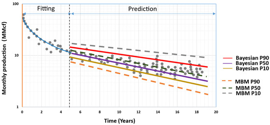
Gong (2011)	Bayesian Analysis	MCMC MH	2000	25 min	Approximate posterior
Gonzalez (2012)	Bayesian Analysis	MCMC MH	1000	25 min	Approximate posterior
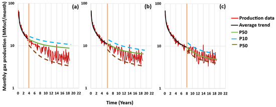
Fanchi (2013)	Bayesian Analysis	MC	1000	-	Uniform
Kim (2014)	Bayesian Analysis	MC	5000	-	Triangle
Zhukovsky (2016)	Bayesian Analysis	MCMC MH	100,000	25 min	Approximate posterior
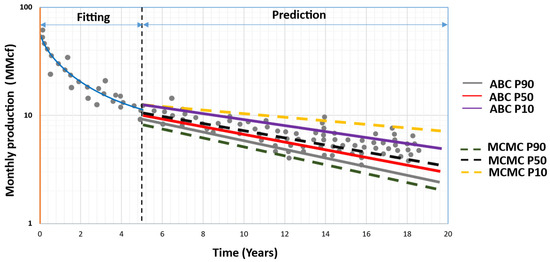
Paryani (2017)	Bayesian Analysis	MCMC ABC MC ABC Rejection ABC	10,000	Faster than Gong (2011)	Likelihood-free approximation
Jimenez (2017)	Bayesian Analysis	MC	-	-	Chi-square
Joshi (2018)	Frequentist Analysis	Time series
Hong (2019)	Bayesian Analysis	MC	-	-	Uniform
Fanchi (2020)	Bayesian Analysis	MC	1000	-	Uniform
Korde (2021)	Bayesian Analysis	MCMC Gibbs MH ABC	20,000	5–25 s	Likelihood
pDCA Model	The Study Domain			The Combined DCA Model(s)	Reference
Jochen (1996)	Conventional oil wells, two different fields			Arps	^[10]
Cheng (2010)	Conventional mature oil and gas wells; 100 wells			Arps	^[11]
Minin (2011)	Shale gas reservoirs; 150 gas wells			Arps	^[13]
Brito (2012)	Conventional oil wells			PDE	^[14]
Gong (2011)	Shale gas reservoirs; 197 gas wells			Arps	^[12]
Gonzalez (2012)	Shale gas reservoirs; 197 gas wells			Arps, PLE, SEPD, and Duong	^[9]
Fanchi (2013)	Shale gas reservoirs; 110 gas wells			Arps and SEPD	^[16]
Kim (2014)	Shale gas reservoirs; 4 gas wells			Arps, SEPD, and PDE	^[17]
Zhukovsky Approach (2016)	Shale reservoirs; 199 shale oil wells			EEDCA	^[18]
Paryani (2017)	Unconventional reservoirs; 21 oil wells (Eagle Ford) and 100 gas wells (Barnett Shale)			Arps and LGM	^[19]^[20]
Jimenez Approach (2017)	Tight gas reservoir; 1 gas well			Arps, SEPD, PLE, LGM, and Duong	^[21]
Joshi Approach (2018)	Shale reservoirs; 100 shale gas wells			LGM and SEPD	^[22]
Hong (2019)	Unconventional shale oil; Bakken field, 28 wells, and Midland field, 31 wells			Arps, SEPD, LGM, and Pan	^[23]
Fanchi (2020)	Unconventional shale oil; Bakken field, 9 wells, and Eagle Ford, 6 wells			Arps and SEPD	^[24]
Korde (2021)	Conventional and unconventional reservoirs; 23 oil wells and 51 gas wells			Arps, SEPD, PLE, Duong, and LGM	^[25]

References

Liang, H.-B.; Zhang, L.-H.; Zhao, Y.-L.; Zhang, B.-N.; Chang, C.; Chen, M.; Bai, M.-X. Empirical Methods of Decline-Curve Analysis for Shale Gas Reservoirs: Review, Evaluation, and Application. J. Nat. Gas Sci. Eng. 2020, 83, 103531.
Joshi, K.; Lee, J. Comparison of Various Deterministic Forecasting Techniques in Shale Gas Reservoirs. In Proceedings of the SPE Hydraulic Fracturing Technology Conference, The Woodlands, TX, USA, 4–6 February 2013; OnePetro: Richardson, TX, USA, 2013.
Yehia, T.; Khattab, H.; Tantawy, M.; Mahgoub, I. Removing the Outlier from the Production Data for the Decline Curve Analysis of Shale Gas Reservoirs: A Comparative Study Using Machine Learning. ACS Omega 2022, doi:10.1021/acsomega.2c03238.
Chen, Q.; Wang, N.; Ruan, K.; Zhang, M. Selection of Production Decline Analysis Method of Shale Gas Well. Reserv. Eval. Dev. 2018, 8, 76–79.
Mahmoud, O. Machine Learning Outlier Detection Algorithms for Enhancing Production Data Analysis of Shale Gas Machine Learning Outlier Detection Algorithms for Enhancing Production Data Analysis of Shale Gas. In; 2023; pp. 127–163 ISBN 978-81-19-21749-6. https://doi.org/10.9734/bpi/fraps/v4/6060A
Yehia, T.; Wahba, A.; Mostafa, S.; Mahmoud, O. Suitability of Different Machine Learning Outlier Detection Algorithms to Improve Shale Gas Production Data for Effective Decline Curve Analysis. Energies 2022, 15, 8835, doi:10.3390/en15238835.
Yuan, J.; Luo, D.; Feng, L. A Review of the Technical and Economic Evaluation Techniques for Shale Gas Development. Appl. Energy 2015, 148, 49–65.
Yehia, T.; Khattab, H.; Tantawy, M.; Mahgoub, I. Improving the Shale Gas Production Data Using the Angular- Based Outlier Detector Machine Learning Algorithm. JUSST 2022, 24, 152–172, doi:http://doi.org/10.51201/JUSST/22/08150.
Gonzalez, R.; Gong, X.; McVay, D. Probabilistic decline curve analysis reliably quantifies uncertainty in shale gas reserves regardless of stage of depletion. In Proceedings of the SPE Eastern Regional Meeting, Lexington, KY, USA, 3–5 October 2012.
Jochen, V.A.; Spivey, J.P. Probabilistic Reserves Estimation Using Decline Curve Analysis with the Bootstrap Method. In Proceedings of the SPE Annual Technical Conference and Exhibition, Denver, CO, USA, 6 October 1996; OnePetro: Richardson, TX, USA, 1996.
Cheng, Y.; Wang, Y.; McVay, D.A.A.; Lee, W.J.J. Practical Application of a Probabilistic Approach to Estimate Reserves Using Production Decline Data. SPE Econ. Manag. 2010, 2, 19–31.
Gong, X.; Gonzalez, R.; McVay, D.A.; Hart, J.D. Bayesian Probabilistic Decline-Curve Analysis Reliably Quantifies Uncertainty in Shale-Well-Production Forecasts. SPE J. 2014, 19, 1047–1057.
Minin, A.; Guerra, L.; Colombo, I. Unconventional Reservoirs Probabilistic Reserve Estimation Using Decline Curves. In Proceedings of the International Petroleum Technology Conference, Bangkok, Thailand, 15 November 2011; p. IPTC-14801-MS.
Brito, L.E.; Paz, F.; Belisario, D. Probabilistic Production Forecasts Using Decline Envelopes. In Proceedings of the SPE Latin America and Caribbean Petroleum Engineering Conference, Mexico City, Mexico, 16 April 2012; p. SPE-152392-MS.
Gong, X.; Gonzalez, R.; McVay, D.; Hart, J. Bayesian Probabilistic Decline Curve Analysis Quantifies Shale Gas Reserves Uncertainty. In Proceedings of the Canadian Unconventional Resources Conference, Calgary, AB, Canada, 15 November 2011; p. SPE-147588-MS.
Fanchi, J.R.; Cooksey, M.J.; Lehman, K.M.; Smith, A.; Fanchi, A.C.; Fanchi, C.J. Probabilistic Decline Curve Analysis of Barnett, Fayetteville, Haynesville, and Woodford Gas Shales. J. Pet. Sci. Eng. 2013, 109, 308–311.
Kim, J.-S.; Shin, H.-J.; Lim, J.-S. Application of a Probabilistic Method to the Forecast of Production Rate Using a Decline Curve Analysis of Shale Gas Play. In Proceedings of the Twenty-Fourth International Ocean and Polar Engineering Conference, Busan, Republic of Korea, 15–20 June 2014; p. ISOPE-I-14-158.
Zhukovsky, I.D.; Mendoza, R.C.; King, M.J.; Lee, W.J. Uncertainty Quantification in the EUR of Eagle Ford Shale Wells Using Probabilistic Decline-Curve Analysis with a Novel Model. In Proceedings of the Abu Dhabi International Petroleum Exhibition & Conference, Abu Dhabi, United Arab Emirates, 7 November 2016; p. D021S049R005.
Paryani, M. Approximate Bayesian Computation for Probabilistic Decline Curve Analysis in Unconventional Reservoirs. Master’s Thesis, University of Alaska Fairbanks, College, AK, USA, 2015. Available online: https://hdl.handle.net/11122/6383 (accessed on 15 December 2022).
Paryani, M.; Awoleke, O.O.; Ahmadi, M.; Hanks, C.; Barry, R. Approximate Bayesian Computation for Probabilistic Decline-Curve Analysis in Unconventional Reservoirs. SPE Reserv. Eval. Eng. 2017, 20, 478–485.
Jiménez, E.T.; Cervantes, R.J.; Magnelli, D.E.; Dabrowski, A. Probabilistic Approach of Advanced Decline Curve Analysis for Tight Gas Reserves Estimation Obtained from Public Data Base. In Proceedings of the SPE Latin America and Caribbean Petroleum Engineering Conference, Buenos Aires, Argentina, 17 May 2017; p. D021S009R006.
Joshi, K.G.; Awoleke, O.O.; Mohabbat, A. Uncertainty Quantification of Gas Production in the Barnett Shale Using Time Series Analysis. In Proceedings of the SPE Western Regional Meeting, Garden Grove, CA, USA, 22 April 2018; OnePetro: Richardson, TX, USA, 2018.
Hong, A.; Bratvold, R.B.; Lake, L.W.; Ruiz Maraggi, L.M. Integrating Model Uncertainty in Probabilistic Decline-Curve Analysis for Unconventional-Oil-Production Forecasting. SPE Reserv. Eval. Eng. 2019, 22, 861–876.
Fanchi, J. Decline Curve Analysis of Shale Oil Production Using a Constrained Monte Carlo Technique. J. Basic Appl. Sci. 2020, 16, 61–67.
Korde, A.; Goddard, S.D.; Awoleke, O.O. Probabilistic Decline Curve Analysis in the Permian Basin Using Bayesian and Approximate Bayesian Inference. SPE Reserv. Eval. Eng. 2021, 24, 536–551.
Yehia, T.; Naguib, A.; Abdelhafiz, M.M.; Hegazy, G.M.; Mahmoud, O. Probabilistic Decline Curve Analysis: State-of-the-Art Review. Energies 2023, 16, 4117, doi:10.3390/en16104117.

© Text is available under the terms and conditions of the Creative Commons Attribution (CC BY) license; additional terms may apply. By using this site, you agree to the Terms and Conditions and Privacy Policy.

Upload a video for this entry

Information

Subjects: Engineering, Petroleum

Contributors MDPI registered users' name will be linked to their SciProfiles pages. To register with us, please refer to https://encyclopedia.pub/register :

Taha Yehia

Ahmed Naguib

Mostafa M. Abdelhafiz

Gehad M. Hegazy

Omar Mahmoud

View Times: 422

Update Date: 12 Jun 2023

Table of Contents

Video Upload Options

Confirm

1. Introduction