Machine Learning in Healthcare Industry

Version	Summary	Created by	Modification	Content Size	Created at	Operation
1		Angela An	--	2668	2023-05-04 21:48:07	\|
2	format corrected.	Beatrix Zheng	Meta information modification	2668	2023-05-05 16:14:53	\| \|
3	format corrected.	Beatrix Zheng	Meta information modification	2668	2023-05-05 16:15:46	\|

This entry is adapted from the peer-reviewed paper 10.3390/s23094178

Machine learning is a mechanism that enables machines to learn automatically without explicit programming. The main area of machine learning is to use advanced algorithms and statistical techniques to access the data and predict accuracy instead of a rule-based system. The dataset is a primary component of machine learning accuracy prediction. As a result, the data are more relevant and the prediction is more accurate. Machine learning has been used in different fields, such as finance, retail, and the healthcare industry. The rising use of machine learning in healthcare provides more opportunities for disease diagnosis and treatment. Machine learning has a great feature of continuous improvement for data accurate prediction and classification purposes for disease analysis.

machine learning machine learning algorithms healthcare mobile health

1. Overview of Machine-Learning in Healthcare

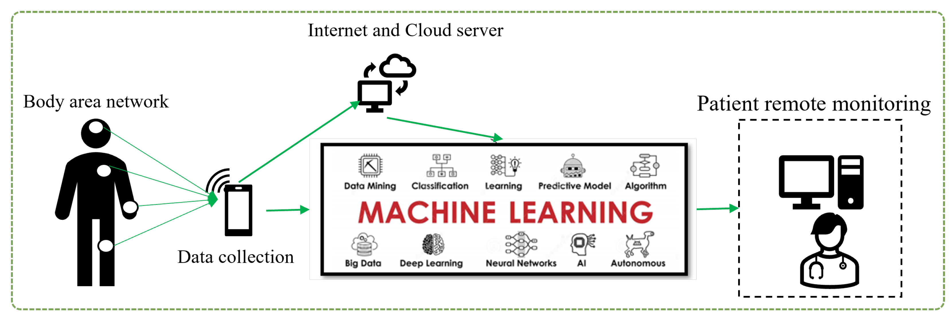
Machine learning is a type of artificial intelligence that involves training algorithms on data so that they can make predictions or take actions without being explicitly programmed. In healthcare, machine learning has the potential to revolutionize how we diagnose, treat, and prevent diseases, as shown in Figure 1. Some potential applications of machine learning in healthcare include:

Figure 1. Concept of machine learning in healthcare area.

Predictive analytics: Machine learning algorithms can analyze data from electronic health records, claims data and other sources to predict the likelihood of specific health outcomes, such as hospital readmissions or the onset of chronic diseases. This can help healthcare providers identify high-risk patients and take proactive steps to prevent adverse outcomes.
Diagnosis and treatment: Machine learning algorithms can be trained to analyze medical images, such as CT scans or X-rays, to help diagnose or identify the most appropriate treatment for a patient.
Personalized medicine: Machine learning can be used to predict which treatments are most likely to be effective for a given patient based on their individual characteristics, such as their genetics and medical history.
Clinical decision support: Machine learning algorithms can be integrated into clinical decision support systems to help healthcare providers make more informed decisions about patient care.
Population health management: Machine learning can be used to analyze data from large populations to identify trends and patterns that can inform the development of public health initiatives.

Overall, the use of machine learning in healthcare has the potential to improve patient outcomes, reduce costs, and enhance the efficiency of the healthcare system.

2. Overview of Machine Learning

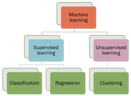
Machine learning can be categorized into two categories: supervised learning and unsupervised learning, shown in Figure 2. Supervised machine learning trains the algorithms on known input and output data to predict future outputs. Unsupervised machine learning discovers hidden patterns or internal structures within the input data. Supervised machine learning can perform both classifications and regression tasks, while unsupervised machine learning tackles the clustering tasks ^[1].

Figure 2. Types of machine learning such as supervised and unsupervised learning.

2.1. Some Common Supervised Classification Machine Learning Algorithms

Supervised machine learning classification techniques are algorithms that predict a categorical outcome called classification, the given data are labelled and known compared to unsupervised learning. The input data are categorised into training, and testing data ^[2]. The classification algorithms predict discrete responses by classifying the input data into categories. The classical supervised machine learning application includes heart attack prediction, medical image processing, and speech recognition ^[1]. Supervised learning derives classification models from these training data. These models can then be used to perform classification on other unlabelled data. The training dataset includes an output variable that needs to be classified. All algorithms learn specific patterns from the training data and apply them to the test data for a classification problem ^[1]. Some well-known supervised classification machine learning algorithms are decision trees, support vector machines, naïve Bayes, K-nearest neighbors, and neural networks.

The general machine learning architecture is shown in Figure 3 and the details of this step are described as follows:

Figure 3. The general architecture of machine learning with requires steps such as data to feature extraction and training to prediction using different machine learning models.

2.1.1. Health Datasets

Healthcare datasets are comprehensive collections of information related to patients’ health. These datasets typically contain a broad range of data points, including medical history, diagnostic test results, medication usage, and demographic information. They serve various purposes, such as clinical research, public health monitoring, and quality improvement initiatives. Examples of healthcare datasets include electronic health records (EHRs), which are digital records of patient’s medical information, and claims datasets, which provide information about healthcare services received and their associated costs. Additionally, there are disease registries that contain data on individuals with specific diseases or conditions, and clinical trial datasets that contain information on participants, interventions, and outcomes. Healthcare datasets are complex and can be challenging to analyze due to their size and complexity. Nevertheless, researchers can use advanced analytical techniques such as machine learning and natural language processing to gain insights into patient health outcomes and develop targeted interventions to improve patient care.

2.1.2. Feature Extractions

Selecting the most relevant features from a dataset is a crucial component of machine learning known as feature extraction ^[3]. Feature extraction involves transforming the raw data into features that possess a strong ability to recognize patterns. In this process, the original data are considered to have weak recognition ability compared to the extracted features ^[4]. The objective of this process is to identify the vital attributes or traits from the original data that will serve as inputs for a machine learning algorithm to execute a specific task. Numerous methods are available for feature extraction, including principal component analysis (PCA) ^[5], linear discriminant analysis (LDA) ^[6], t-distributed stochastic neighbor embedding (t-SNE) ^[7], autoencoders ^[8], filter methods ^[9], and wrapper methods ^[10].

PCA: PCA is a widely used dimensionality reduction method in data analysis and machine learning. As a linear transformation approach, it aims to discern patterns in high-dimensional data by projecting it onto a lower-dimensional space. The primary objective of PCA is to encapsulate the most important variations in the data while minimizing noise and redundancy ^[5].
LDA: Linear discriminant analysis (LDA) is a supervised dimensionality reduction method extensively used in machine learning, pattern recognition, and statistical evaluation. LDA’s main goal is to convert high-dimensional data into a lower-dimensional space while optimizing the distinction between different classes. This property makes LDA especially fitting for classification tasks, as well as for extracting features and visualizing multifaceted, multi-class data ^[6].
t-SNE: t-SNE is a non-linear dimensionality reduction method that is especially adept at visualizing high-dimensional data. Laurens van der Maaten and Geoffrey Hinton created t-SNE in 2008. Its primary purpose is to conserve local structures within the data, which entails preserving the distances between adjacent data points during dimensionality reduction. This characteristic renders t-SNE highly effective in unveiling patterns, clusters, and structures within intricate datasets ^[7].
Autoencoders: Autoencoders are a form of unsupervised artificial neural network employed for dimensionality reduction, feature extraction, and representation learning. They comprise an encoder and a decoder that collaboratively compress and reconstructs input data while minimizing information loss. Autoencoders are especially valuable for tasks such as denoising, anomaly detection, and unsupervised pre-training for intricate neural networks ^[8].
Filter methods: these techniques prioritize features by evaluating them using specific statistical metrics such as correlation, mutual information, or the chi-square test. Subsequently, the most prominent features are chosen. Filter methods are exemplified by approaches like Pearson’s correlation and Information Gain (IG) method ^[9].
Wrapper methods: Wrapper methods represent feature selection approaches utilized in machine learning and data analysis. Their main objective is to determine the best subset of features that enhances the performance of a specific machine learning algorithm. By directly evaluating various feature combinations based on the performance of the learning algorithm, wrapper methods are more computationally demanding than filter methods, which are based on the data’s inherent characteristics ^[10].

2.1.3. Decision Trees

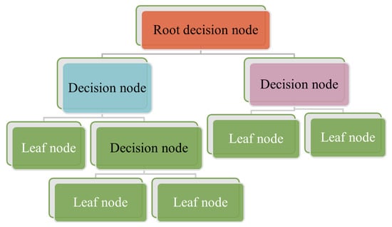
A decision trees classifier uses graphical tree information to demonstrate possible alternatives, outcomes, and end values (Figure 4). This involves a computational process to calculate probabilities in deciding on a few courses of action ^[11]. The decision trees algorithm starts with training data samples and their related category labels. The training set is recursively divided into subsets based on feature values, so the data in each subset is purer than the data in the parent set. Each internal node of the decision tree represents a test feature, whilst every branch node presents the test result, and the leaf nodes present the class label. Since the classifier decision tree is used to identify an unknown sample’s category label, it will be able to track the path from the root node to the leaf nodes and hold the sample’s category label ^[12]. The advantage of the decision tree algorithm is that it is fast and simple, where no domain knowledge or parameter setting is required, and high dimensional data can be handled in the context. Further, decision tree algorithms support incremental learning, which is immutable because of the alternative functions based on each internal node ^[12].

Figure 4. Demonstration of decision trees with the root, decision, and Leaf nodes. Start from the root node, then move to the decision node using the leaf node information.

Building decision trees can be a lengthy process, particularly when working with sizable datasets or a high number of features. This is because the algorithm must evaluate every potential split at each level of the tree, which can be computationally costly ^[13].

Medical experts frequently employ data mining techniques to aid in the diagnosis of cardiac disorders. Regarding sensitivity, specificity, and accuracy, the decision tree is one of the effective machine-learning algorithms for heart attack detection ^[14]. In the medical field, heart disease has been extensively detected and prevented using the decision tree classification technique. Using eight patient data variables and a decision tree, Pathak and Valan were able to predict heart disease with an accuracy of 88% ^[15], while ^[16] used the decision tree for prediction of heart disease. In ^[11], researchers employed decision tree algorithms to reduce the volume of data by converting data into a more condensed form in order to preserve the crucial features and increase accuracy in mobile health technology.

2.1.4. Support Vector Machine (SVM)

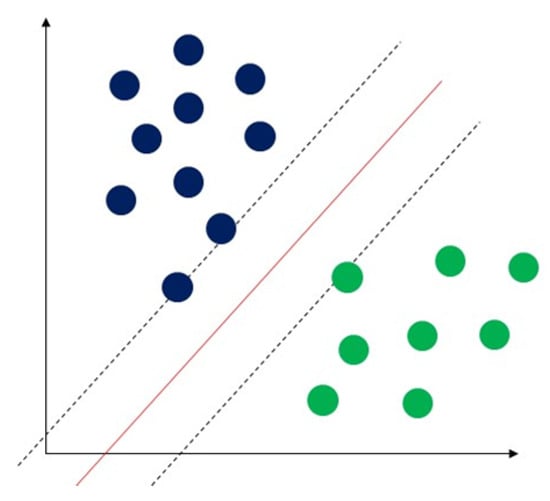
Support vector machine (SVM) is a classical machine learning technique that can address classification problems. Importantly, SVM supports multidomain applications in a big data mining environment ^[17]. SVM uses some model features to train data to generate reliable estimators from a dataset ^[18]. The concept of SVM maximizes the minimum distance from the hyperplane to the nearest point of the sample presented in Figure 5 ^[19].

Figure 5. Demonstration of support vector machine. The solid red line indicates the separating hyperplane and the distance between two dotted lines is the maximum margin for separating different classes.

SVM produces higher performance when dealing with a large dataset than other pattern recognition algorithms, such as Bayesian networks, etc. Additionally, one main advantage of SVM is that its data training is comparatively easy (Pradhan, 2012). Most importantly, according to (Bhavsar and Ganatra, 2012), SVM provides high accuracy among machine learning algorithms. The disadvantage of SVM is that it is exceedingly slow in machine learning, as a large amount of training time is needed. Further, memory requirements increase with the square of the number of training examples ^[20]. SVM is one of the most effective machine learning algorithms for pattern recognition. Most SVM applications are used for facial recognition, illness detection and prevention, speech recognition, image recognition, and facial detection ^[21]. Some authors have used an improved stacked SVM for early heart failure (HF) prediction in medical applications. Their findings demonstrated that the model has superior performance with an accuracy range from 57.85% and 91.83% ^[22]. In a different study, fuzzy support vector machines were utilized to make diagnoses of coronary heart disease. Experiments revealed that, when compared to non-incremental learning technology, this technique significantly sped up illness diagnosis computation time ^[23].

2.1.5. Naïve Bayes

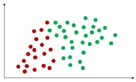
Naïve Bayes is one of the most widely used classification algorithms. The assumption of naïve Bayes only includes one parent node and a few independent child nodes rendering it the simplest Bayesian network ^[24]. Naive Bayes (NB) uses the probability classification method by multiplying the individual probability of each attribute-value pair, as shown in Figure 6. This simple algorithm presumes independence between attributes and provides remarkable classification results ^[25]. One strength of the naïve Bayes algorithm is that it has a short computational data training time ^[26], where classification performance can be improved by removing irrelevant attributes ^[27]. This can lead it to perform better with small datasets and in dealing with multiple classification tasks. In addition to this, naïve Bayes is suitable for incremental training (where it can train supplementary samples in real-time) ^[28]. As the algorithm is not very sensitive to missing data, is relatively simple, and can often be used for text classification, naïve Bayes is easy to understand the interpretation of the results ^[29]. The drawbacks of the naïve Bayes include its lower rate of accuracy compared to other sophisticated supervised machine learning algorithms, such as ANNs. Further, naïve Bayes requires many training records to achieve excellent performance results ^[30]. Since naïve Bayes is very efficient and easy to implement, it is commonly used in text classification, spam filtering, or news classification ^[31]. In the medical field, the naïve Bayes algorithm has been used for disease detection and prediction. One study deployed a naïve Bayes classifier to skin image data for skin disease detection, revealing the results to outperform other methods with accuracy from 91.2 to 94.3% ^[32]. Gupta et al. have used naïve Bayes for heart disease detection through feature selection in the medical sector, with experimental results achieving 88.16% accuracy in the test dataset ^[33].

Figure 6. Demonstration of naïve Bayes with the distribution of different classes.

2.1.6. K-Nearest Neighbours (K-NN)

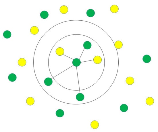
The K-nearest neighbours (K-NN) classification algorithm is one of the simplest methods in data mining classification technology. The assumption of K-NN is to identify an unknown pattern by assigning a value to the K, where the nearest neighbor category of the K training sample is considered the same as the classification illustrated in Figure 7 ^[34]. A few factors are involved in the classifier, such as selected K-value and distance measurement, and so on ^[35]. K-NN requires less computational time to train the data than other machine algorithms. However, it requires more computational time in the classification phase ^[20]. The advantage of K-NN is that it is easy to understand and implement for classification. Further to this, it can perform well with many class labels for a dataset. Similarly, the data training stage is faster than other machine learning algorithms ^[20]. The drawbacks of the K-NN are its computational cost, with a sizeable unlabelled sample, and time delay during the classification phase. Apart from cross-validation, k-NN also lacks the principles to sign a K’s value and is expensive computationally. Further, confusion may occur if too many unrelated attributes are in the data, leading to poor accuracy ^[20]. K-NN is also frequently utilized for disease detection and diagnosis ^[36]. K-NN is one of the most used data mining approaches for classification problems, and researchers have tried to utilize it to help medical professionals diagnose heart disease ^[37]. To identify heart disease, for instance, some researchers have developed a unique algorithm that combines K-NN and genetic algorithms in an effort to increase the accuracy of prediction ^[36]. Shouman et al. studied whether incorporating other algorithms into K-NNs can improve accuracy in the diagnosis of cardiac disease. According to their findings, using K-NN instead of a neural network could increase the accuracy of diagnosis of heart disease ^[37]. The summary of existing supervised learning performance in terms of accuracy in the healthcare industry using classification algorithms is presented in Table 1.

Figure 7. Demonstration of K-NN identifying unknown pattern by assigning a value to the K, where the nearest neighbor category of the K training sample is considered the same as the classification.

Table 1. Summary of existing supervised learning performance in terms of accuracy in the healthcare industry using classification algorithms.

Classification Algorithms	Reference	Year	Task	Accuracy
Decision trees	^[15]	2020	Heart disease prediction	88%
	^[11]	2012	Data volume reduction	80/32%
	^[16]	2001	Hear disease prediction	81.11%
Support vector machine (SVM)	^[22]	2019	Facial recognition, illness detection and prevention, speech recognition, image recognition, and facial detection	57.85–91.3%
Naïve Bayes	^[32]	2020	Skin disease detection	91.2–94.3%
	^[33]	2020	Heart disease detection	88.16%
	^[16]	2001	Hear disease prediction	81.48%
K-nearest neighbours (K-NN)	^[36]	2013	Heart disease diagnosis	75.8–100%
	^[37]	2012	Heart disease diagnosing	94–97.1%

References

Ciaburro, G.; Iannace, G.; Ali, M.; Alabdulkarem, A.; Nuhait, A. An artificial neural network approach to modelling absorbent asphalts acoustic properties. J. King Saud. Univ. Eng. Sci. 2021, 33, 213–220.
Das, S.; Dey, A.; Pal, A.; Roy, N. Applications of artificial intelligence in machine learning: Review and prospect. Int. J. Comput. Appl. 2015, 115, 31–41.
Muna, A.H.; Moustafa, N.; Sitnikova, E. Identification of malicious activities in industrial internet of things based on deep learning models. J. Inf. Secur. Appl. 2018, 41, 1–11.
Cai, J.; Luo, J.; Wang, S.; Yang, S. Feature selection in machine learning: A new perspective. Neurocomputing 2018, 300, 70–79.
Song, F.; Guo, Z.; Mei, D. Feature selection using principal component analysis. In Proceedings of the 2010 International Conference on System Science, Engineering Design and Manufacturing Informatization, Yichang, China, 12–14 November 2010; Volume 1, pp. 27–30.
Wen, J.; Fang, X.; Cui, J.; Fei, L.; Yan, K.; Chen, Y.; Xu, Y. Robust sparse linear discriminant analysis. IEEE Trans. Circuits Syst. Video Technol. 2018, 29, 390–403.
Li, M.A.; Luo, X.Y.; Yang, J.F. Extracting the nonlinear features of motor imagery EEG using parametric t-SNE. Neurocomputing 2016, 218, 371–381.
Luo, X.; Li, X.; Wang, Z.; Liang, J. Discriminant autoencoder for feature extraction in fault diagnosis. Chemom. Intell. Lab. Syst. 2019, 192, 103814.
Nagarajan, S.M.; Muthukumaran, V.; Murugesan, R.; Joseph, R.B.; Meram, M.; Prathik, A. Innovative feature selection and classification model for heart disease prediction. J. Reliab. Intell. Environ. 2022, 8, 333–343.
Li, B.; Zhang, P.l.; Tian, H.; Mi, S.S.; Liu, D.S.; Ren, G.Q. A new feature extraction and selection scheme for hybrid fault diagnosis of gearbox. Expert Syst. Appl. 2011, 38, 10000–10009.
Mohamed, W.N.H.W.; Salleh, M.N.M.; Omar, A.H. A comparative study of reduced error pruning method in decision tree algorithms. In Proceedings of the 2012 IEEE International Conference on Control System, Computing and Engineering, Penang, Malaysia, 23–25 November 2012; pp. 392–397.
Kotsiantis, S.B.; Zaharakis, I.; Pintelas, P. Supervised machine learning: A review of classification techniques. Emerg. Artif. Intell. Appl. Comput. Eng. 2007, 160, 3–24.
Ray, S. A quick review of machine learning algorithms. In Proceedings of the 2019 International Conference on Machine Learning, Big Data, Cloud and Parallel Computing (COMITCon), Faridabad, India, 14–16 February 2019; pp. 35–39.
Thenmozhi, K.; Deepika, P. Heart disease prediction using classification with different decision tree techniques. Int. J. Eng. Res. Gen. Sci. 2014, 2, 6–11.
Pathak, A.K.; Arul Valan, J. A predictive model for heart disease diagnosis using fuzzy logic and decision tree. In Smart Computing Paradigms: New Progresses and Challenges; Springer: Berlin/Heidelberg, Germany, 2020; pp. 131–140.
Cheung, N. Machine Learning Techniques for Medical Analysis; School of Information Technology and Electrical Engineering: Atlanta, GA, USA, 2001.
Suthaharan, S. Support vector machine. In Machine Learning Models and Algorithms for Big Data Classification; Springer: Berlin/Heidelberg, Germany, 2016; pp. 207–235.
Kazemi, M.; Kazemi, K.; Yaghoobi, M.A.; Bazargan, H. A hybrid method for estimating the process change point using support vector machine and fuzzy statistical clustering. Appl. Soft Comput. 2016, 40, 507–516.
Yuan, R.; Li, Z.; Guan, X.; Xu, L. An SVM-based machine learning method for accurate internet traffic classification. Inf. Syst. Front. 2010, 12, 149–156.
Bhavsar, H.; Ganatra, A. A comparative study of training algorithms for supervised machine learning. Int. J. Soft Comput. Eng. (IJSCE) 2012, 2, 2231–2307.
Boero, L.; Marchese, M.; Zappatore, S. Support vector machine meets software defined networking in ids domain. In Proceedings of the 2017 29th International Teletraffic Congress (ITC 29), Genoa, Italy, 4–8 September 2017; Volume 3, pp. 25–30.
Ali, L.; Niamat, A.; Khan, J.A.; Golilarz, N.A.; Xingzhong, X.; Noor, A.; Nour, R.; Bukhari, S.A.C. An optimized stacked support vector machines based expert system for the effective prediction of heart failure. IEEE Access 2019, 7, 54007–54014.
Nilashi, M.; Ahmadi, H.; Manaf, A.A.; Rashid, T.A.; Samad, S.; Shahmoradi, L.; Aljojo, N.; Akbari, E. Coronary heart disease diagnosis through self-organizing map and fuzzy support vector machine with incremental updates. Int. J. Fuzzy Syst. 2020, 22, 1376–1388.
Arar, Ö.F.; Ayan, K. A feature dependent Naive Bayes approach and its application to the software defect prediction problem. Appl. Soft Comput. 2017, 59, 197–209.
Nasteski, V. An overview of the supervised machine learning methods. Horizons. B 2017, 4, 51–62.
Dulhare, U.N. Prediction system for heart disease using Naive Bayes and particle swarm optimization. Biomed. Res. 2018, 29, 2646–2649.
Mydyti, H. Data Mining Approach Improving Decision-Making Competency along the Business Digital Transformation Journey: A Case Study–Home Appliances after Sales Service. Seeu Rev. 2021, 16, 45–65.
Abikoye, O.C.; Omokanye, S.O.; Aro, T.O. Text Classification Using Data Mining Techniques: A Review. Comput. Inf. Syst. J. 2018, 1, 1–8.
Berrar, D. Bayes’ theorem and naive bayes classifier. In Encyclopedia of Bioinformatics and Computational Biology: ABC of Bioinformatics; Elsevier Science Publisher: Amsterdam, The Netherlands, 2018; Volume 403, p. 412.
Osisanwo, F.; Akinsola, J.; Awodele, O.; Hinmikaiye, J.; Olakanmi, O.; Akinjobi, J. Supervised machine learning algorithms: Classification and comparison. Int. J. Comput. Trends Technol. (IJCTT) 2017, 48, 128–138.
Xu, S. Bayesian Naïve Bayes classifiers to text classification. J. Inf. Sci. 2018, 44, 48–59.
Balaha, H.M.; Hassan, A.E.S. Skin cancer diagnosis based on deep transfer learning and sparrow search algorithm. Neural Comput. Appl. 2023, 35, 815–853.
Gupta, A.; Kumar, L.; Jain, R.; Nagrath, P. Heart disease prediction using classification (naive bayes). In Proceedings of the First International Conference on Computing, Communications, and Cyber-Security (IC4S 2019), Chandigarh, India, 12 October 2019; pp. 561–573.
Duneja, A.; Puyalnithi, T. Enhancing classification accuracy of k-nearest neighbours algorithm using gain ratio. Int. Res. J. Eng. Technol 2017, 4, 1385–1388.
Chen, Z.; Zhou, L.J.; Da Li, X.; Zhang, J.N.; Huo, W.J. The Lao text classification method based on KNN. Procedia Comput. Sci. 2020, 166, 523–528.
Deekshatulu, B.; Chandra, P. Classification of heart disease using k-nearest neighbor and genetic algorithm. Procedia Technol. 2013, 10, 85–94.
Shouman, M.; Turner, T.; Stocker, R. Applying k-nearest neighbour in diagnosing heart disease patients. Int. J. Inf. Educ. Technol. 2012, 2, 220–223.

© Text is available under the terms and conditions of the Creative Commons Attribution (CC BY) license; additional terms may apply. By using this site, you agree to the Terms and Conditions and Privacy Policy.

Upload a video for this entry

Information

Subjects: Computer Science, Artificial Intelligence

Contributors MDPI registered users' name will be linked to their SciProfiles pages. To register with us, please refer to https://encyclopedia.pub/register :

View Times: 617

Update Date: 05 May 2023

Table of Contents

Video Upload Options

Confirm