Your browser does not fully support modern features. Please upgrade for a smoother experience.
Submitted Successfully!
 +1 credit
Thank you for your contribution! You can also upload a video entry or images related to this topic.
For video creation, please contact our Academic Video Service.
| Version | Summary | Created by | Modification | Content Size | Created at | Operation |
|---|---|---|---|---|---|---|
| 1 | Bradley John Roth | -- | 2281 | 2023-05-03 11:55:42 | | | |
| 2 | Camila Xu | Meta information modification | 2281 | 2023-05-04 02:52:17 | | |
Video Upload Options
We provide professional Academic Video Service to translate complex research into visually appealing presentations. Would you like to try it?
Cite
If you have any further questions, please contact Encyclopedia Editorial Office.
Roth, B.J. The Magnetoencephalogram. Encyclopedia. Available online: https://encyclopedia.pub/entry/43700 (accessed on 24 June 2026).
Roth BJ. The Magnetoencephalogram. Encyclopedia. Available at: https://encyclopedia.pub/entry/43700. Accessed June 24, 2026.
Roth, Bradley J.. "The Magnetoencephalogram" Encyclopedia, https://encyclopedia.pub/entry/43700 (accessed June 24, 2026).
Roth, B.J. (2023, May 03). The Magnetoencephalogram. In Encyclopedia. https://encyclopedia.pub/entry/43700
Roth, Bradley J.. "The Magnetoencephalogram." Encyclopedia. Web. 03 May, 2023.
Copy Citation
In 1968, biomagnetism pioneer David Cohen performed the first measurement of the magnetic field of the brain: the magnetoencephalogram (MEG). He detected the brain’s largest signal: the alpha rhythm. This nearly sinusoidal oscillation at a frequency of about 10 Hz is turned on or off by closing or opening your eyes.
biomagnetism
inverse problem
magnetocardiogram
magnetoencephalogram
1. First Measurements of the Magnetoencephalogram
In 1968, biomagnetism pioneer David Cohen performed the first measurement of the magnetic field of the brain: the magnetoencephalogram (MEG). He detected the brain’s largest signal: the alpha rhythm [1]. This nearly sinusoidal oscillation at a frequency of about 10 Hz is turned on or off by closing or opening your eyes. Since this experiment was performed before SQUID magnetometers were introduced into biomagnetism, Cohen wound a million-turn pickup coil to record the MEG. He averaged 2500 times by triggering off the electroencephalogram (EEG). Subsequent studies used a SQUID magnetometer to sense the approximately 1 pT magnetic field [2].
The MEG is primarily produced by currents in the dendrites of neurons in the brain [3][4]. Magnetic fields evoked in these neurons by a stimulus are about ten times weaker than those associated with the alpha rhythm and are a thousand times weaker than the magnetocardiogram. The visual-evoked magnetic field was detected by Sam Williamson and his colleagues in 1975 [5]. By using a second-order gradiometer, they were able to record a 0.1 pT signal in their laboratory in downtown Manhattan, with no shielded room. Similar results were obtained by Cohen’s group [6] and others [7]. Soon, evoked magnetic fields were observed during electrical stimulation of the finger [8], following voluntary finger flexion [9][10], and in response to a sound [11][12][13][14][15][16]. MEG recordings were sensitive enough to demonstrate how distinct regions in the brain responded to different sound frequencies: tonotopic organization [17].
2. Magnetic Field of a Dipole in a Spherical Conductor
The initial calculations of the magnetic field underlying the magnetoencephalogram were performed assuming that the head is a sphere [18][19][20]. An influential article by Jukka Sarvas, from the biomagnetism group in Finland, summarized three essential facts about the magnetic field of a dipole in a spherical conductor [21], as follows:
-
A radial dipole produces no magnetic field (Figure 1). This result is best proven using Ampere’s law: the magnetic field integrated along a closed loop is proportional to the net current threading the loop. The symmetry is sufficient that the integral over the path (dashed circle in Figure 1) equals the path length times the magnetic field. The current produced by a dipole, including the return current, must be contained within the sphere because the region outside is not conducting. Hence, the net current threading the loop (dipole plus return current) is zero, so the magnetic field of a radial dipole vanishes.
-
The radial component of the magnetic field is the same as for a dipole in a homogenous, unbounded conductor. In other words, the conductor–insulator interface at the surface of the sphere does not affect the radial component of the magnetic field. Furthermore, this result holds for a heterogeneous sphere, as long as the conductivity varies only with depth. For these reasons, investigators prefer measuring the radial component of the magnetic field when studying the MEG.
-
The tangential component of the magnetic field is affected by the conductor–insulator boundary, but it does not depend on a conductivity that radially varies.
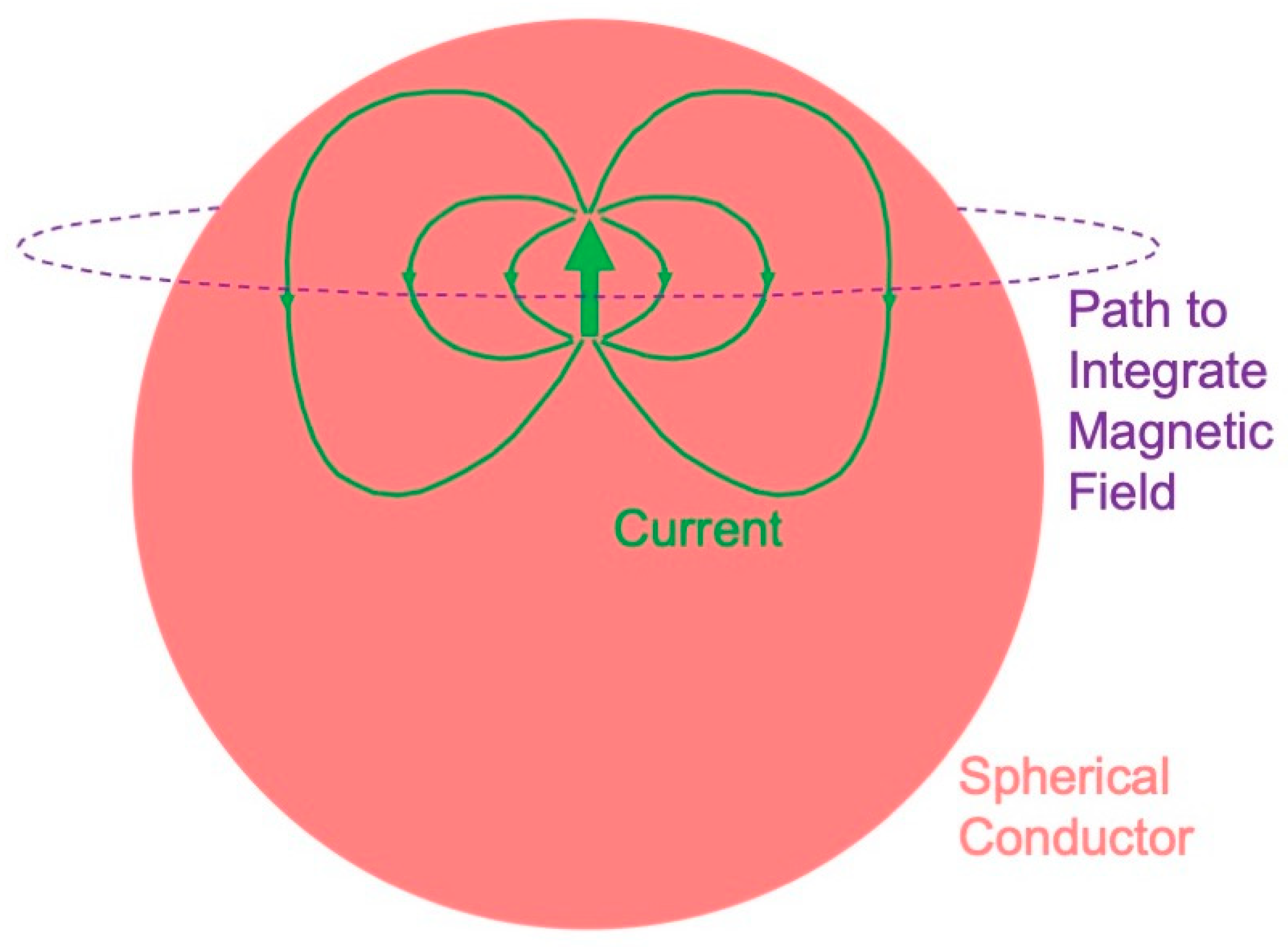
Figure 1. The magnetic field of a radial dipole is zero outside a spherical conductor.
These results have a significance for the magnetoencephalogram. You cannot record a magnetic field from radial dipoles, such as those that may exist in cortical folds or gyri [22]—they are magnetically silent. The electroencephalogram does have a signal from a radial dipole, so an advantage of the EEG over MEG is that the EEG detects radial sources. The three-sphere model—consisting of concentric spheres representing the brain, skull, and scalp—is often used to model the head. The magnetoencephalogram is independent of a conductivity that radially varies, so it does not depend on the low conductivity of the skull. The electroencephalogram is dramatically influenced by the skull conductivity, so an advantage of the MEG over the EEG is that the MEG is independent of the skull, scalp, and brain conductivities. Numerical calculations [23][24][25] and phantom studies [26][27][28][29][30] show that these conclusions that were rigorously proven for a sphere are good, but not perfect, approximations for a realistically shaped head.
3. Relative Merits of the Magnetoencephalogram and the Electroencephalogram
The last section analyzed some of the relative merits of the magnetoencephalogram and the electroencephalogram. Are there enough advantages of the MEG over the EEG to justify the cost and complexity of cryogenics? The magnetic field pattern is rotated by 90° relative to the electrical voltage distribution, so the MEG should provide better localization perpendicular to a dipole, while the EEG should better localize parallel to it. In addition, the MEG might reveal tangential dipoles that are obscured in the EEG by radial ones [31].
In 1990, Cohen created a stir by claiming that the MEG did not localize a source better than EEG did [32]. He and his coworkers implanted dipoles at known locations in the brains of patients undergoing seizure monitoring. When they solved the inverse problem to determine the location of the dipole from either electric or magnetic data, they found each had a localization error of about 10 mm. Critics such as Sam Williamson [33] and a team led by Riitta Hari [34] claimed that Cohen’s study was limited by obsolete equipment and poor procedures. Wikswo, Williamson, and Alan Gevins weighed the pros and cons of the two techniques [35]. Measuring the EEG is less expensive than the MEG and does not require as extensive shielding. The patient is able to move while recording the EEG because the electrodes are attached to the scalp, but the head has to be motionless when measuring the MEG. The MEG is less affected than the EEG if you pick a wrong value of the skull conductivity when solving the inverse problem.
By the mid-1990s, the MEG was becoming an established technique for investigating brain activity. In 1993, Matti Hämäläinen and his collaborators in Finland surveyed magnetoencephalography in the Reviews of Modern Physics [36]. It is the most highly cited publication in the field of biomagnetism and continues to provide one of the best summaries of MEG theory, instrumentation, and applications.
4. Solving the Inverse Problem
How to solve the inverse problem—determining the sources of brain activity from magnetic measurements—is the central question in magnetoencephalography. In general, the solution is not unique. For example, if you assume a spherical head, then you may always add a radial dipole to any solution [21]. In addition, the inverse solution is often not stable. Slight measurement errors propagate through an algorithm to cause major errors in the calculated sources. In other words, the problem is ill-posed, which means that “trusting the data too much will unquestionably lead to nonsense solutions” [37].
The inverse problem was initially solved for a single dipole. Its location, orientation, and strength were determined by a least-squares fit to the experimental data. The technique can be generalized to multiple dipoles [38][39], but with too many the algorithm becomes underdetermined: the number of source parameters exceeds the number of data points. In this case, numerous solutions might provide equally good fits and a method is needed to select the optimal one. A common method is to select the minimum-norm solution: the solution having the least magnitude squared when summed over all dipoles. The least-squares minimum-norm solution is found using singular-value decomposition [40][41].
Often, least-squares minimum-norm methods are applied at one instant. If solved at different times, the resulting dipoles could move or rotate. An alternative approach is to assume a few fixed dipoles that each produce their own individual (asynchronous) time series. The fit is performed over their postulated locations and time (spatial-temporal analysis). John Mosher and Richard Leahy have applied this multiple-signal classification (MUSIC) algorithm, and a recursively applied and projected MUSIC algorithm (RAP-MUSIC), to MEG data [42][43][44].
The MUSIC algorithm has been generalized by employing spatial filtering (beamformers), where the filter emphasizes regions of interest within the brain while attenuating other locations [45][46]. Beamformers are best-suited for studying processes that are coherent in time but are spatially segregated. An advantage of this algorithm is that you do not have to make any assumption about the number of sources.
Still another approach to solving the MEG inverse problem is to use known anatomical and physiological constraints. The least-squares minimum-norm fit is performed subject to these constraints by adopting a Bayesian formulation to produce a “maximum a posteriori” estimate of brain activity [37]. One implementation of this technique is known as low-resolution electromagnetic tomography (LORETA) [37][47][48]. Such procedures require that the MEG data be integrated with anatomical information from other methods, such as MRI.
If you have no anatomical information, or you do not wish to form any hypotheses about the source, you can go to the other extreme and construct a solution that directly relates the magnetic field to the current, bypassing any restrictive assumptions or least-squares fit. Similarly, Hämäläinen and Risto Ilmoniemi related the current in the brain to the magnetic field measured outside a spherical head, reducing the inverse problem to a linear estimation [49]. To keep their problem well-posed, they had to apply a minimum-norm constraint and a regularization procedure. This technique predicts current distributions that explain the MEG data with hardly any a priori assumptions [50][51]. The solutions tend to be diffuse, and the procedure often poorly localizes restricted sources.
A variation of linear estimation for the inverse problem is the focal underdetermined system solution (FOCUSS) [52]. The algorithm starts with a minimum-norm solution and then recursively strengthens the sources in some regions and suppresses them in others, until they exist in only a small number of locations. The weightings that determine which regions are strengthened or suppressed are found from previous iterations, so the algorithm tends to focus on a handful of sources. This algorithm is particularly useful when there is reason to suspect that the MEG is produced by a few, well-localized sites. Norman Tepley and his team have developed a multi-resolution version of FOCUSS that uses wavelets to make the algorithm less susceptible to noise [53][54].
This entry cannot examine all the various algorithms for solving the inverse problem, there are just too many. For example, whole families of methods are based on coherence [55] and connectivity [56][57]. One of the most promising ways to contribute to MEG research is to further develop novel solutions to the inverse problem. It remains an important barrier limiting the use of MEG in medicine.
5. Clinical Applications
Magnetoencephalography is able to diagnose and help treat many illnesses. Daniel Barth and his coworkers at UCLA used MEG to localize interictal spikes: transient, brief discharges, often observed in patients with epilepsy [58]. Such spikes occur in the same tissue as seizures originate from, so localization of the source of interictal spikes assists surgeons who perform brain surgery to treat epilepsy [59]. A clinical study of over 1000 participants provided some of the most impressive evidence yet for the utility of MEG in epilepsy diagnosis. It indicated that MEG “provides non-redundant information, which significantly contributes to patient selection, focus localization and ultimately long-term seizure freedom after epilepsy surgery” [60].
In addition to epilepsy, magnetoencephalography has other medical applications [61]. It has proven useful when diagnosing patients with impaired visual word processing due to dyslexia [62]. The data suggest that dyslexics have difficulty with written words because the parts of the left temporal lobe responsible for auditory language are impaired. Patients with Parkinson’s disease suffer from tremor, and MEG data indicate that involuntary activation of what is normally voluntary motor activity may trigger the tremor [63]. Direct current MEG demonstrates that depression-like activity spreads during migraine aura, which may cause the occipital cortex to become hyperexcitable [64]. Recordings of spontaneous MEG activity suggest that depression, tinnitus, neurogenic pain, and Parkinson’s disease may all be caused by a dysrhythmia in the interaction of the brain’s thalamus and cortex [65]. Even deep brain structures such as the hippocampus and amygdala can be monitored with MEG [66]. Sylvain Baillet of McGill University has reviewed the applications of MEG, and he expects it “to play an increasing and pivotal role in the elucidation of these grand mechanistic principles of cognitive, systems and clinical neuroscience” [67].
One way to encourage medical doctors to adopt MEG techniques is to make them easier and cheaper. SQUIDs constructed using high-temperature superconductors may allow the coolant to be liquid nitrogen instead of the more expensive and difficult to handle liquid helium [68][69]. Enormous shielded rooms sometimes might be replaced by active shielding, where the current passed through external coils cancels out extraneous magnetic field noise [70]. Software such as “brainstorm” [71] and “MNE” [72] is facilitating the use of MEG by clinicians. Artificial intelligence and deep learning are increasingly assisting doctors in interpreting the MEG [73].
Both the MEG and EEG must compete with other methods for imaging the brain, such as functional magnetic resonance imaging (fMRI) and positron emission tomography (PET). MEG and EEG provide better temporal resolution than fMRI and PET, but fMRI and PET provide better spatial resolution and do not require solving an ill-posed inverse problem. Although MEG is more expensive than EEG, it is not as expensive as fMRI or PET. Traditional MEG, similar to fMRI and PET, is completely non-contact (EEG requires attaching electrodes to the head, which may be difficult in some cases such as when there is damage to the scalp). MEG and EEG do not require injecting any radioactive isotopes into the patient, as PET does. fMRI measures blood flow in the brain and PET measures metabolic activity, whereas MEG and EEG directly record brain electrical activity. Ultimately, combinations of these techniques may be used together to learn more about how the brain works.
References
- Cohen, D. Magnetoencephalography: Evidence of magnetic fields produced by alpha-rhythm currents. Science 1968, 161, 784–786.
- Cohen, D. Magnetoencephalography: Detection of the brain’s electrical activity with a superconducting magnetometer. Science 1972, 175, 664–666.
- Okada, Y.C.; Wu, J.; Kyuhou, S. Genesis of MEG signals in a mammalian CNS structure. Electroencephalogr. Clin. Neurophysiol. 1997, 103, 474–485.
- Murakami, S.; Okada, Y. Contributions of principal neocortical neurons to magnetoencephalography and electroencephalography signals. J. Physiol. 2006, 575, 925–936.
- Brenner, D.; Williamson, S.J.; Kaufman, L. Visually evoked magnetic fields of the human brain. Science 1975, 190, 480–482.
- Teyler, T.J.; Cuffin, B.N.; Cohen, D. The visual evoked magnetoencephalogram. Life Sci. 1975, 17, 683–691.
- Reite, M.; Zimmerman, J.E.; Edrich, J.; Zimmerman, J. The human magnetoencephalogram: Some EEG and related correlations. Electroencephalogr. Clin. Neurophysiol. 1976, 40, 59–66.
- Brenner, D.; Lipton, J.; Kaufman, L.; Williamson, S.J. Somatically evoked magnetic fields of the human brain. Science 1978, 199, 81–83.
- Okada, Y.C.; Williamson, S.J.; Kaufman, L. Magnetic field of the human sensorimotor cortex. Int. J. Neurosci. 1982, 17, 33–38.
- Cheyne, D.; Weinberg, H. Neuromagnetic fields accompanying unilateral finger movements: Pre-movement and movement-evoked fields. Exp. Brain Res. 1989, 78, 604–612.
- Reite, M.; Edrich, J.; Zimmerman, J.T.; Zimmerman, J.E. Human magnetic auditory evoked fields. Electroencephalogr. Clin. Neurophysiol. 1978, 45, 114–117.
- Hari, R.; Aittoniemi, K.; Järvinen, M.-L.; Katila, T.; Varpula, T. Auditory evoked transient and sustained magnetic fields of the human brain localization of neural generators. Exp. Brain Res. 1980, 40, 237–240.
- Hari, R.; Kaila, K.; Katila, T.; Tuomisto, T.; Varpula, T. Interstimulus interval dependence of the auditory vertex response and its magnetic counterpart: Implications for their neural generation. Electroencephalogr. Clin. Neurophysiol. 1982, 54, 561–569.
- Hari, R.; Reinikainen, K.; Kaukoranta, E.; Hämäläinen, M.; Ilmoniemi, R.; Penttinen, A.; Salminen, J.; Teszner, D. Somatosensory evoked cerebral magnetic fields from SI and SII in man. Electroencephalogr. Clin Neurophysiol. 1984, 57, 254–263.
- Hari, R.; Hämäläinen, M.; Ilmoniemi, R.; Kaukoranta, E.; Reinikainen, K.; Salminen, J.; Alho, K.; Näätänen, R.; Sams, M. Responses of the primary auditory cortex to pitch changes in a sequence of tone pips: Neuromagnetic recordings in man. Neurosci. Lett. 1984, 50, 127–132.
- Pantev, C.; Makeig, S.; Hoke, M.; Galambos, R.; Hampson, S.; Gallen, C. Human auditory evoked gamma-band magnetic fields. Proc. Natl. Acad. Sci. USA 1991, 88, 8996–9000.
- Romani, G.L.; Williamson, S.J.; Kaufman, L. Tonotopic organization of the human auditory cortex. Science 1982, 216, 1339–1340.
- Grynszpan, F.; Geselowitz, D.B. Model studies of the magnetocardiogram. Biophys. J. 1973, 13, 911–925.
- Cuffin, B.N.; Cohen, D. Magnetic fields of a dipole in special volume conductor shapes. IEEE Trans. Biomed. Eng. 1977, 24, 372–381.
- Cohen, D.; Cuffin, B.N. Demonstration of useful differences between magnetoencephalogram and electroencephalogram. Electroencephalogr. Clin. Neurophysiol. 1983, 56, 38–51.
- Sarvas, J. Basic mathematical and electromagnetic concepts of the biomagnetic inverse problem. Phys. Med. Biol. 1987, 32, 11–22.
- Kaufman, L.; Kaufman, J.H.; Wang, J.-Z. On cortical folds and neuromagnetic fields. Electroencephalogr. Clin. Neurophysiol. 1991, 79, 211–226.
- Hämäläinen, M.S.; Sarvas, J. Feasibility of the homogeneous head model in the interpretation of neuromagnetic fields. Phys. Med. Biol. 1987, 32, 91–97.
- Hämäläinen, M.S.; Sarvas, J. Realistic conductivity geometry model of the human head for interpretation of neuromagnetic data. IEEE Trans Biomed Eng. 1989, 36, 165–171.
- Meijs, J.W.H.; Bosch, F.G.C.; Peters, M.J.; Lopes da Silva, F.H. On the magnetic field distribution generated by a dipolar current source situated in a realistically shaped compartment model of the head. Electroencephalogr. Clin. Neurophysiol. 1987, 66, 286–298.
- Weinberg, H.; Brickett, P.; Coolsma, F.; Baff, M. Magnetic localisation of intracranial dipoles: Simulation with a physical model. Electroencephalogr. Clin. Neurophysiol. 1986, 64, 159–170.
- Barth, D.S.; Sutherling, W.; Broffman, J.; Beatty, J. Magnetic localization of a dipolar current source implanted in a sphere and a human cranium. Electroencephalogr. Clin. Neurophysiol. 1986, 63, 260–273.
- Rose, D.F.; Ducla-Soares, E.; Sato, S. Improved accuracy of MEG localization in the temporal region with inclusion of volume current effects. Brain Topogr. 1989, 1, 175–181.
- Leahy, R.M.; Mosher, J.C.; Spencer, M.E.; Huang, M.X.; Lewine, J.D. A study of dipole localization accuracy for MEG and EEG using a human skull phantom. Electroencephalogr. Clin. Neurophysiol. 1998, 107, 159–173.
- Okada, Y.C.; Lahteenmäki, A.; Xu, C. Experimental analysis of distortion of magnetoencephalography signals by the skull. Clin. Neurophysiol. 1999, 110, 230–238.
- Cuffin, B.N.; Cohen, D. Comparison of the magnetoencephalogram and electroencephalogram. Electroencephalogr. Clin. Neurophysiol. 1979, 47, 132–146.
- Cohen, D.; Cuffin, B.N.; Yunokuchi, K.; Maniewski, R.; Purcell, C.; Cosgrove, G.R.; Ives, J.; Kennedy, J.G.; Schomer, D.L. MEG versus EEG localization test using implanted sources in the human brain. Ann. Neurol. 1990, 28, 811–817.
- Williamson, S.J. MEG versus EEG localization test. Ann. Neurol. 1991, 30, 222.
- Hari, R.; Hämäläinen, M.; Ilmoniemi, R.; Lounasmaa, O.V. Comment on “MEG versus EEG localization test using implanted sources in the human brain”. Ann. Neurol. 1991, 30, 222–223.
- Wikswo, J.P.; Gevins, A.; Williamson, S.J. The future of EEG and MEG. Electroencephalogr. Clin. Neurophysiol. 1993, 87, 1–9.
- Hämäläinen, M.; Hari, R.; Ilmoniemi, R.J.; Knuutila, J.; Lounasmaa, O.V. Magnetoencephalography: Theory, instrumentation, and applications to noninvasive studies of the working human brain. Rev. Mod. Phys. 1993, 65, 413–497.
- Baillet, S.; Garnero, L. A Bayesian approach to introducing anatomo-functional priors in the EEG/MEG inverse problem. IEEE Trans. Biomed. Eng. 1997, 44, 374–385.
- Ueno, S.; Iramina, K. Modeling and source localization of MEG activities. Brain Topogr. 1990, 3, 151–165.
- Iramina, K.; Ueno, S. Source estimation of spontaneous MEG activity and auditory evoked responses in normal subjects during sleep. Brain Topogr. 1996, 8, 297–301.
- Wang, J.-Z.; Williamson, S.J.; Kaufman, L. Magnetic source images determined by a lead-field analysis: The unique minimum-norm least-squares estimation. IEEE Trans. Biomed. Eng. 1992, 39, 665–675.
- Jeffs, B.; Leahy, R.; Singh, M. An evaluation of methods for neuromagnetic image reconstruction. IEEE Trans. Biomed. Eng. 1987, 34, 713–723.
- Mosher, J.C.; Lewis, P.S.; Leahy, R.M. Multiple dipole modeling and localization from spatio-temporal MEG data. IEEE Trans. Biomed. Eng. 1992, 39, 541–557.
- Mosher, J.C.; Leahy, R.M. Recursive MUSIC: A framework for EEG and MEG source localization. IEEE Trans. Biomed. Eng. 1998, 45, 1342–1354.
- Mosher, J.C.; Leahy, R.M. Source localization using recursively applied and projected (RAP) MUSIC. IEEE Trans. Signal Process. 1999, 47, 332–340.
- van Veen, B.D.; van Drongelen, W.; Yuchtman, M.; Suzuki, A. Localization of brain electrical activity via linearly constrained minimum variance spatial filtering. IEEE Trans. Biomed. Eng. 1997, 44, 867–880.
- Hillebrand, A.; Singh, K.D.; Holliday, I.E.; Furlong, P.L.; Barnes, G.R. A new approach to neuroimaging with magnetoencephalography. Hum. Brain Mapp. 2005, 25, 199–211.
- Pascual-Marqui, R.D. Standardized low resolution brain electromagnetic tomography (sLORETA): Technical details. Methods Find. Exp. Clin. Pharmacol. 2002, 24, 5–12.
- Pascual-Marqui, R.D.; Esslen, M.; Lehmann, D. Functional imaging with low resolution brain electromagnetic tomography (LORETA): A review. Methods Find. Exp. Clin. Pharmacol. 2002, 24, 91–95.
- Hämäläinen, M.S.; Ilmoniemi, R.J. Interpreting magnetic fields of the brain: Minimum norm estimates. Med. Biol. Eng. Comput. 1994, 32, 35–42.
- Ioannides, A.A.; Bolton, J.P.R.; Clarke, C.J.S. Continuous probabilistic solutions to the biomagnetic inverse problem. Inverse Probl. 1990, 6, 523–542.
- Ribary, U.; Ioannides, A.A.; Singh, K.D.; Hasson, R.; Bolton, J.P.; Lado, F.; Mogilner, A.; Llinás, R. Magnetic field tomography of coherent thalamocortical 40-Hz oscillations in humans. Proc. Natl. Acad. Sci. USA 1991, 88, 11037–11041.
- Gorodnitsky, I.F.; George, J.S.; Rao, B.D. Neuromagnetic source imaging with FOCUSS: A recursive weighted minimum norm algorithm. Electroencephalogr. Clin. Neurophysiol. 1995, 95, 231–251.
- Bowyer, S.M.; Moran, J.E.; Mason, K.M.; Constantinou, J.E.; Smith, B.J.; Barkley, G.L.; Tepley, N. MEG localization of language-specific cortex utilizing MR-FOCUSS. Neurology 2004, 62, 2247–2255.
- Moran, J.E.; Bowyer, S.M.; Tepley, N. Multi-resolution FOCUSS: A source imaging technique applied to MEG data. Brain Topogr. 2005, 18, 1–17.
- Bowyer, S.M. Coherence a measure of brain networks: Past and present. Neuropsychiat. Electrophysiol. 2016, 2, 1.
- Schoffelen, J.-M.; Gross, J. Source connectivity analysis with MEG and EEG. Hum. Brain Mapp. 2009, 30, 1857–1865.
- Hillebrand, A.; Barnes, G.R.; Bosboom, J.L.; Berendse, H.W.; Stam, C.J. Frequency-dependent functional connectivity within resting-state networks: An atlas-based MEG beamformer solution. NeuroImage 2012, 59, 3909–3921.
- Barth, D.S.; Sutherling, W.; Engel, J.; Beatty, J. Neuromagnetic localization of epileptiform spike activity in the human brain. Science 1982, 218, 891–894.
- Rose, D.F.; Smith, P.D.; Sato, S. Magnetoencephalography and epilepsy research. Science 1987, 238, 329–335.
- Rampp, S.; Stefan, H.; Wu, X.; Kaltenhäuser, M.; Maess, B.; Schmitt, F.C.; Wolters, C.H.; Hamer, H.; Kasper, B.S.; Schwab, S.; et al. Magnetoencephalography for epileptic focus localization in a series of 1000 cases. Brain 2019, 142, 3059–3071.
- Hari, R.; Salmelin, R. Magnetoencephalograhy: From SQUIDs to neuroscience: Neuroimage 20th anniversary special edition. NeuroImage 2012, 61, 386–396.
- Salmelin, R.; Kiesilä, P.; Uutela, K.; Service, E.; Solonen, O. Impaired visual word processing in dyslexia revealed with magnetoencephalography. Ann. Neurol. 1996, 40, 157–162.
- Volkmann, J.; Joliot, M.; Mogilner, A.; Ioannides, A.A.; Lado, F.; Fazzini, E.; Ribary, U.; Llinás, R. Central motor loop oscillations in parkinsonian resting tremor revealed by magnetoencephalography. Neurology 1996, 46, 1359–1370.
- Bowyer, S.M.; Aurora, S.K.; Moran, J.E.; Tepley, N.; Welch, K.M.A. Magnetoencephalographic fields from patients with spontaneous and induced migraine aura. Ann. Neurol. 2001, 50, 582–587.
- Llinás, R.R.; Ribary, U.; Jeanmonod, D.; Kronberg, E.; Mitra, P.P. Thalamocortical dysrhythmia: A neurological and neuropsychiatric syndrome characterized by magnetoencephalography. Proc. Natl. Acad. Sci. USA 1999, 96, 15222–15227.
- Pizzo, F.; Roehri, N.; Villalon, S.M.; Trébuchon, A.; Chen, S.; Lagarde, S.; Carron, R.; Gavaret, M.; Giusiano, B.; McGonigal, A.; et al. Deep brain activities can be detected with magnetoencephalography. Nat. Commun. 2019, 10, 971.
- Baillet, S. Magnetoencephalography for brain electrophysiology and imaging. Nat. Neurosci. 2017, 20, 327–339.
- Koelle, D.; Kleiner, R.; Ludwig, F.; Dantsker, E.; Clarke, J. High-transition-temperature superconducting quantum interference devices. Rev. Mod. Phys. 1999, 71, 631–686.
- Faley, M.I.; Dammers, J.; Maslennikov, Y.V.; Schneiderman, J.F.; Winkler, D.; Koshelets, V.P.; Shah, N.J.; Dunin-Borkowki, R.E. High-Tc SQUID biomagnetometers. Supercond. Sci. Technol. 2017, 30, 083001.
- Romani, G.L.; Williamson, S.J.; Kaufman, L. Biomagnetic instrumentation. Rev. Sci. Instrum. 1982, 53, 1815–1845.
- Tadel, F.; Baillet, S.; Mosher, J.C.; Pantazis, D.; Leahy, R.M. Brainstorm: A user-friendly application for MEG/EEG analysis. Comput. Intell. Neurosci. 2011, 2011, 879716.
- Gramfort, A.; Luessi, M.; Larson, E.; Engemann, D.A.; Strohmeier, D.; Brodbeck, C.; Parkkonen, L.; Hämäläinen, M.S. MNE software for processing MEG and EEG data. NeuroImage 2014, 86, 446–460.
- Pantazis, D.; Adler, A. MEG source localization via deep learning. Sensors 2021, 21, 4278.
More
Information
Subjects:
Biophysics
Contributor
MDPI registered users' name will be linked to their SciProfiles pages. To register with us, please refer to https://encyclopedia.pub/register
:
View Times:
1.4K
Revisions:
2 times
(View History)
Update Date:
04 May 2023
Table of Contents


Notice
You are not a member of the advisory board for this topic. If you want to update advisory board member profile, please contact office@encyclopedia.pub.
OK
Confirm
Only members of the Encyclopedia advisory board for this topic are allowed to note entries. Would you like to become an advisory board member of the Encyclopedia?
Yes
No
${ textCharacter }/${ maxCharacter }
Submit
Cancel
Back
Comments
${ item }
|
${ item.createdUser.fullName }
${ item.createdAt }
${ item.vote }
${ item.reply }
Delete
${ reply.createdUser.fullName }
${ reply.createdAt }
${ reply.vote }
Delete
There is no reply to this comment~
${ item.replyTextCharacter }/${ item.replyMaxCharacter }
Submit
Cancel
More
No more~
There is no comment~
${ textCharacter }/${ maxCharacter }
Submit
Cancel
${ selectedItem.replyTextCharacter }/${ selectedItem.replyMaxCharacter }
Submit
Cancel
Confirm
Are you sure to Delete?
Yes
No