 +1 credit
| Version | Summary | Created by | Modification | Content Size | Created at | Operation |
|---|---|---|---|---|---|---|
| 1 | Sergey Borovik | -- | 6384 | 2023-01-10 11:42:33 | | | |
| 2 | Jason Zhu | Meta information modification | 6384 | 2023-01-11 03:20:38 | | | | |
| 3 | Jason Zhu | Meta information modification | 6384 | 2023-01-13 04:03:25 | | |
Video Upload Options
Single-coil eddy current sensors (SCECS) form a separate and independent branch among the existing eddy current probes. Such sensors are often used for aviation and aerospace applications where the conditions accompanying the measuring process are harsh and even extreme. High temperatures (up to +600 °C in the compressor and over +1000 °C in the turbine of gas turbine engines), the complex shape surfaces of the monitored parts, the multidimensional movement of the power plants’ structural elements, restrictions on the probes number and their placement in the measuring zone are the main factors affecting the reliability and accuracy of the measurement results obtained by the sensors. The application of SCECS-based systems in industrial and bench conditions made it possible to identify most of these factors and determine the ways to, if not completely eliminate, then significantly reduce their impact. The effectiveness of the considered approaches and methods has been proven in laboratories and in bench tests of power plants for various purposes. At the same time, many of the proposed solutions are not limited only to SCECS-based systems and can be successfully applied in measurement systems that use other types of eddy-current probes, as well as sensors built on other physical principles.
1. SCECS: Typical Design and Principle of Operation
-
SCECS with SE as the whole current-carrying coil (circuit);
-
SCECS with SE as a fragment of the coil (for example, a segment of a linear conductor).
2. Factors Affecting SCECS: Types and Features of the Influence
2.1. Influence of the Specifics of the Monitored Object
2.2. Electromagnetic Influence on SCECS Constructive Elements
3. SCECS Signals Conversion with Acceptable SNR and Uninformative Parameters Suppression
4. Reducing the Temperature Effect on the SCECS Informative Parameter
 where L0 is the self-inductance of the SCECS (to simplify it is assumed that SCECS1 and SCECS2 are completely similar in their parameters and therefore Ls1 = Ls2 = L0); ΔL is the change in the SCECS inductances caused by the movement of the target in the sensitivity zone of the working sensor. So, the Blumlein bridge provides an almost linear conversion, and the instability of the inductance L does not have a significant impact on the result [32].
5. Specifics of the Monitored Object Design: Impact and Ways to Reduce It
5.1. Consideration of the Complex Surface Shape of Monitored Objects
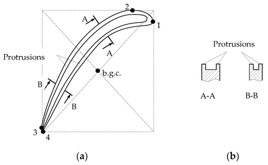
5.2. Protection from the Influence of the Adjacent Elements of the Monitored Object Design on the Result of SCECS Signals Conversion
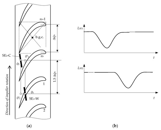
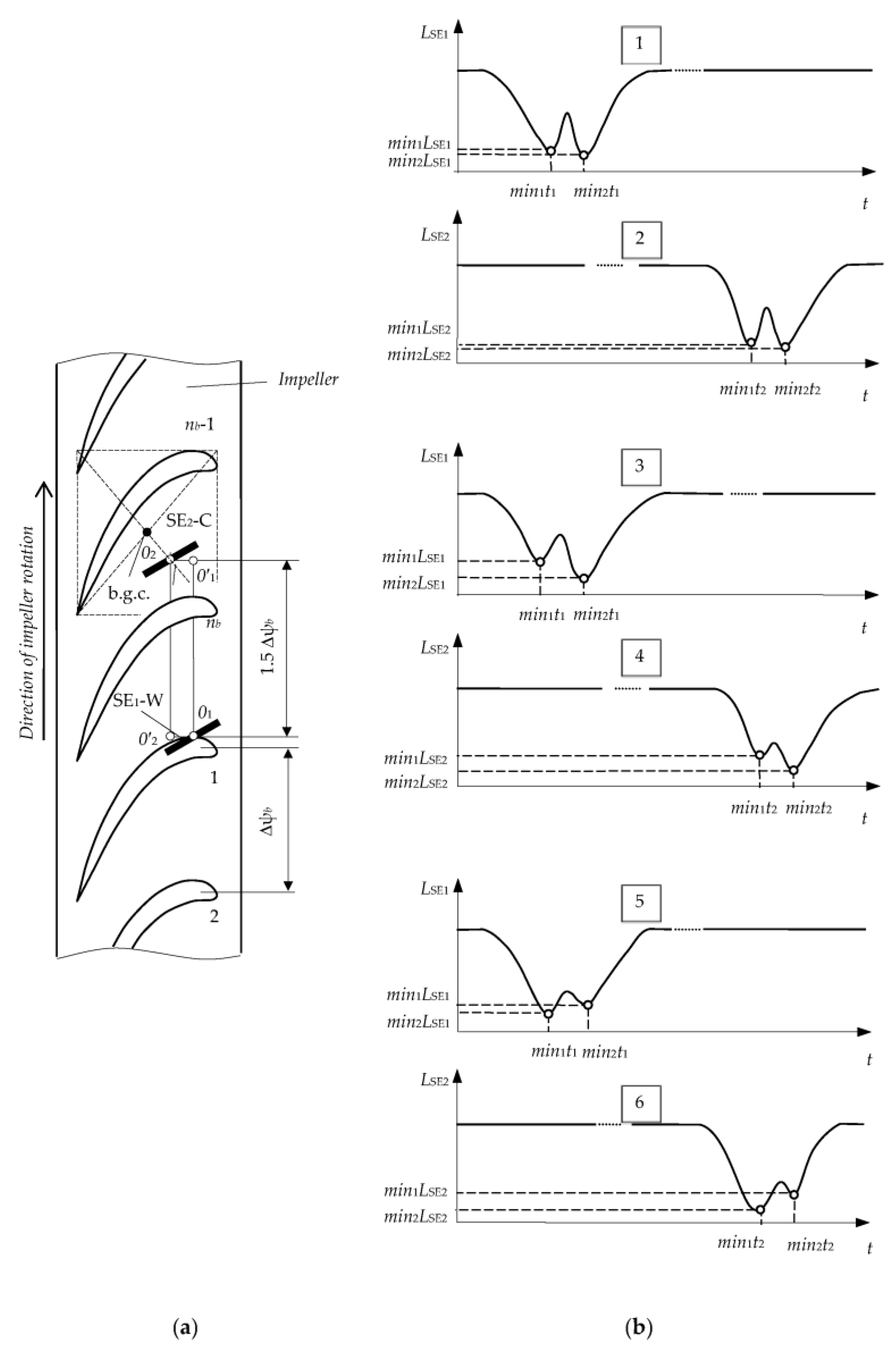
6. SCECS Sampling Synchronization Errors: Causes, Influence, and Ways to Reduce It
References
- Raykov, B.K.; Sekisov, Y.N.; Skobelev, O.P.; Khritin, A.A. Clearance eddy current sensors with sensitive elements the form of a segment of a conductor. Devices Control Syst. 1996, 8, 27–30.
- Borovik, S.; Sekisov, Y. Single-coil eddy current sensors and their application for monitoring the dangerous states of gas-turbine engines. Sensors 2020, 20, 2107.
- Belosludtsev, V.; Borovik, S.; Danilchenko, V.; Sekisov, Y. Wear diagnostics of the thrust bearing of NK-33 turbo-pump unit on the basis of single-coil eddy current sensors. Sensors 2021, 21, 3463.
- Belopukhov, V.; Blinov, A.; Borovik, S.; Luchsheva, M.; Muhutdinov, F.; Podlipnov, P.; Sazhenkov, A.; Sekisov, Y. Monitoring metal wear particles of friction pairs in the oil systems of gas turbine power plants. Energies 2022, 15, 4896.
- Skobelev, O.P.; Sekisov, Y.N.; Khritin, A.A. High-Temperature Conductor Eddy-Current. Converter. Patent SU No. 1394912 A1, 21 October 1986.
- Clarke, C.A.; Larsen, W.E. Aircraft Electromagnetic Compatibility, NASA Report No. DOT/FAA/CT-86/40. 1987. Available online: https://ntrs.nasa.gov/api/citations/19870014423/downloads/19870014423.pdf (accessed on 13 December 2022).
- Williams, T. EMC. In Instrumentation Reference Book, 4th ed.; Boyes, W., Ed.; Butterworth-Heinemann: Oxford, UK, 2010; pp. 797–871.
- Zhao, G.F.; Ying, J.; Wu, L.; Feng, Z.H. Eddy current displacement sensor with ultrahigh resolution obtained through the noise suppression of excitation voltage. Sens. Actuators A Phys. 2019, 299, 111622.
- Lattime, S.; Steinetz, B. Turbine Engine Clearance Control Systems: Current Practices and Future Directions. In Proceedings of the 38th AIAA/ASME/SAE/ASEE Joint Propulsion Conference & Exhibit, Indianapolis, Indiana, 7–10 July 2022.
- Belopukhov, V.N.; Borovik, S.Y.; Kuteynikova, M.M.; Podlypnov, P.E.; Sekisov, Y.N.; Skobelev, O.P. The method for measuring of radial clearances in gas-turbine engine with selfcompensation of temperature effect on sensor. Sens. Syst. 2018, 4, 53–59.
- Zubchenko, A.S.; Koloskov, M.M.; Kashirskiy, Y.V. Steels and Alloys Grade Guide; Zubchenko, A.S., Ed.; Izd. Innovatsionnoe Mashinostroenie: Moscow, Russia, 2021; 672p.
- Shahwaz, M.; Nath, P.; Sen, I. A critical review on the microstructure and mechanical properties correlation of additively manufactured nickel-based superalloys. J. Alloy. Compd. 2022, 907, 164530.
- Sekisov, Y.N.; Skobelev, O.P.; Belenki, L.B.; Borovik, S.Y.; Raykov, B.K.; Slepnev, A.V.; Tulupova, V.V. Methods and Tools for Measuring Multidimensional Displacements of Structural Components of Power Plants; Sekisov, Y.N., Skobelev, O.P., Eds.; Izd. SamNTs RAN: Samara, Russian, 2001; 188p.
- Belenki, L.B.; Raykov, B.K.; Sekisov, Y.N.; Skobelev, O.P. Single-Coil Eddy Current Sensors: From Cluster Compositions to Cluster Constructions. In Proceedings of the VI International Conference “Complex Systems: Control and Modelling Problems”, Samara, Russian, 14–17 June 2004.
- Sridhar, V.; Chana, K.; Pekris, M. High Temperature Eddy Current Sensor System for Turbine Blade Tip Clearance Measurements. In Proceedings of the 12th European Conference on Turbomachinery Fluid dynamics & Thermodynamics (ETC12), Stockholm, Sweden, 3–7 April 2017.
- Zhao, Z.; Liu, Z.; Lyu, Y.; Gao, Y. Experimental investigation of high temperature resistant inductive sensor for blade tip clearance measurement. Sensors 2019, 19, 61.
- Kuteynikova, M.M. Cluster Methods and Tools for Measuring the Radial Clearances and Axial Displacements of the Blade Tips in the Turbine on the Base of Single-Coil Eddy Current Sensors. Ph.D. Thesis, Samara State Technical University, Samara, Russia, 2016.
- Belenki, L.B.; Borovik, S.Y.; Raykkov, B.K.; Sekisov, Y.N.; Skobelev, O.P.; Tulupova, V.V. Cluster Methods and Tools for Measuring Stator Deformations and Displacement Coordinates of Blade Tips in Gas Turbine Engines; Skobelev, O.P., Ed.; Izd. Mashinostroenie: Moscow, Russia, 2011; p. 298.
- Borovik, S.Y.; Kuteynikova, M.M.; Raykov, B.K.; Sekisov, Y.N.; Skobelev, O.P. Method for measuring radial and axial displacements of complex-shaped blade tips. Optoelectron. Instrum. Data Process. 2015, 51, 302–309.
- Borovik, S.; Sekisov, Y. Single-Coil Eddy Current Sensors. In Sensors, Measurements and Networks; Book Series: Advances in Sensors; Yurish, S.Y., Ed.; IFSA Publishing, S.L.: Barcelona, Spain, 2022; Volume 8, pp. 19–48.
- Borovik, S.Y.; Sekisov, Y.N.; Skobelev, O.P. Generalized representation of the methods for obtaining measurement information about the coordinates of the displacements of the blades and propellers tips. Mekhatronika Avtom. Upr. 2007, 3, 19–24.
- Belenki, L.B.; Borovik, S.Y.; Logvinov, A.V.; Raykov, B.K.; Sekisov, Y.N.; Skibelev, O.P.; Tulupova, V.V. Methods for measuring of blade faces displacements in compressors and turbines on basis of distributed clusters of sensors. Part 1. Measurement techniques: Reasoning and description. Mekhatronika Avtom. Upr. 2009, 4, 16–19.
- Borovik, S.Y.; Raykov, B.K.; Sekisov, Y.N.; Skobelev, O.P.; Tulupova, V.V. Method for Measuring the Multidimensional Displacements and Detecting the Vibrations of the Blade Tips of a Turbomachine. Rotor. Patent RF No. 2272990, 27 June 2002.
- Borovik, S.Y.; Kuteynikova, M.M.; Raykov, B.K.; Sekisov, Y.N.; Skobelev, O.P. Measuring of radial clearances between turbine stator and tips of blades with irregular shape by the instrumentality of single-coil eddy-current sensors. Mekhatronika Avtom. Upr. 2013, 10, 38–46.
- Efanov, V.I.; Tihomirov, A.A. Electromagnetic Compatibility of Radio Electronic Means and Systems; Izd. Tomsk State University: Tomsk, Russia, 2012; 228p.
- García-Martín, J.; Gómez-Gil, J.; Vázquez-Sánchez, E. Non-destructive techniques based on eddy current testing. Sensors 2011, 11, 2525–2565.
- Gerasimov, V.G.; Klyuev, V.V.; Shaternikov, V.E. Methods and Devices for Electromagnetic Control; Izd. “Spektr”: Moscow, Russian, 2010; 256p.
- Doebelin, E. Measurement Systems: Applications and Design, 4th ed.; McGraw-Hill Publishing Company: New York City, NY, USA, 1990; 960p.
- Peredelskiy, G.I. Pulse-Powered Bridge Circuits; Energoatomizdat: Moscow, Russia, 1988; 191p.
- Skobelev, O.P. Conversion methods based on test transients. Meas. Control Autom. 1980, 1, 11–17.
- Laplante, P.A. Electrical Engineering Dictionary; CRC Press LLC: Boca Raton, FL, USA, 2000; 380p.
- Nubert, G.P. Measuring Converters of Non-Electric Quantities. In Introduction to the Theory Calculation and Design; Fetisov, M.M., Translator; Energiya: Leningrad, Russia, 1970; 358p.
- Belopukhov, V.N.; Borovik, S.Y.; Kuteynikova, M.M.; Podlypnov, P.E.; Sekisov, Y.N.; Skobelev, O.P. Cluster Methods and Tools for Measuring Radial Clearances in Turbine Flow Section; Skobelev, O.P., Ed.; Izd. Innovatsionnoe Mashinostroenie: Moscow, Russia, 2018; p. 224.
- Carter, B.; Brown, T.R. Handbook of Operational Amplifier Applications; Texas Instruments Incorporated: Dallas, TX, USA, 2001; 94p.
- Belenki, L.B.; Skobelev, O.P. An electronic analogue of the measuring circuit in the form of Blumlein bridge with single-coil eddy current sensors. In Proceedings of the XIII International conference “Complex Systems: Control and Modelling Problems”, Samara, Russian, 15–17 June 2011.
- Peyton, A.J.; Walsh, Y. Analog Electronics with Op Amps: A Source Book of Practical Circuits; Cambridge University Press: Cambridge, UK, 1993; 293p.
- Belenki, L.B.; Skobelev, O.P. Measuring Circuit with Single-Coil Eddy Current Sensors and Approximate Differentiation. In Proceedings of the XIV International Conference “Complex Systems: Control and Modelling Problems”, Samara, Russian, 19–22 June 2012.
- Belenki, L.B.; Kuteynikova, M.M.; Logvinov, A.V.; Sekisov, Y.N.; Skobelev, O.P. Device for Measuring of Multi-Coordinate Displacements of the Blades’. Tips. Patent RF No. 2525614, 27 December 2012.
- Morris, A.S.; Langari, R. Measurement and Instrumentation: Theory and Application, 3d ed.; Academic Press: New York City, NY, USA, 2020; 736p.
- Finkelstein, L. Intelligent and knowledge-based instrumentation. An examination of basic concepts. Measurement 1994, 14, 23–29.
- Podlypnov, P.E. Temperature impact on the controlled and adjacent blades of the compressor impeller when measuring the radial clearances with self-compensation of temperature effects on the sensor. Vestn. SamGTU. Ser. Tekhnicheskie Nauk. 2018, 59, 106–117.
- Belopukhov, V.N.; Borovik, S.Y.; Podlypnov, P.E. Hardware and Software Tools for Automation of Experimental Investigations of the Families of Calibration Characteristics of the Systems for Measuring the Coordinates of Displacements. In Proceedings of the XVI International Conference “Complex Systems: Control and Modelling Problems”, Samara, Russian, 30 June–3 July 2014.
- Borovik, S.Y.; Kuteynikova, M.M.; Sekisov, Y.N.; Skobelev, O.P. Analysis of temperature influence on the informative parameters of single-coil eddy current sensors. Optoelectron. Instrum. Data Process. 2017, 53, 395–401.
- Borovik, S.Y.; Kuteynikova, M.M.; Sekisov, Y.N.; Skobelev, O.P. Influence of turbine wheelspace temperature on measurements of radial and axial displacements of blade tips. Optoelectron. Instrum. Data Process. 2018, 54, 105–111.
- Borovik, S.Y.; Marinina, Y.V.; Sekisov, Y.N. Model of a cluster single-coil eddy current sensor based on the finite element method. Vestn. SamGTU. Ser. Tekhnicheskie Nauk. 2007, 19, 76–83.
- Kuteynikova, M.M.; Sekisov, Y.N. Models of Electromagnetic Interaction of Sensitive Elements of Single-Coil Eddy Current Sensors and Blades. Status and Development. In Proceedings of the XIV International Conference “Complex Systems: Control and Modelling Problems”, Samara, Russian, 19–22 June 2012.
- Borovik, S.Y.; Kuteynikova, M.M.; Sekisov, Y.N.; Skobelev, O.P. Model of the Measuring Circuit with Variable in Time Inductances of Single-Coil Eddy Current Sensors. In Proceedings of the XVI International Conference “Complex Systems: Control and Modelling Problems”, Samara, Russian, 30 June–3 July 2014.
- Borovik, S.Y.; Kuteynikova, M.M.; Podlipnov, P.E.; Sekisov, Y.N.; Skobelev, O.P. Modeling the process of measuring radial and axial displacements of complex-shaped blade tips. Optoelectron. Instrum. Data Process. 2015, 51, 512–522.
- Borovik, S.Y.; Sekisov, Y.N. On the Use of a Thermal Model of a Single-Coil Eddy Current Sensor for the Correction of Temperature Errors. In Proceedings of the VII International Conference “Complex Systems: Control and Modelling Problems”, Samara, Russian, 27 June–1 July 2005.
- NDT Accessories/Zubehör. Product Catalog/Produktkatalog. Release 18b. Available online: https://www.pruftechnik.com/fileadmin/Products-Services/Products/NDT/NDT-Accessories/Encoders-Paint-markers-Warning-units-Test-defect/Downloads/PRUEFTECHNIK_NDT_Accessories_Catalog_EN-DE.pdf (accessed on 13 December 2022).
- Belenki, L.B.; Kuteynikova, M.M.; Raykov, B.K.; Sekisov, Y.N.; Skobelev, O.P. Method for measuring of radial clearances and axial displacements of the blades’ tips of turbine. impeller. Patent RF No. 2457432, 30 December 2010.
- Kaman Instrumentation. High Temperature Displacement System. User Manual. Available online: https://www.kamansensors.com/wp-content/uploads/2016/10/Kaman_High_Temperature_Sensors_manual.pdf (accessed on 23 November 2022).
- Development and Analysis of the Technological Process of Machining of LPT Nozzle Blades. Available online: https://www.turbinist.ru/98-razrabotka-i-analiz-tekhnologicheskogo-processa.html (accessed on 23 November 2022).
- Geykin, V. The perfection of the engine is determined by the perfection of the technology. Engine 2003, 3, 11–15.
- Borovik, S.Y.; Skobelev, O.P. Method errors of the systems for measuring of blade tips radial and axial displacements. Mekhatronika Avtom. Upr. 2012, 4, 31–35.
- Borovik, S.Y. On the error correction of measuring of blades tips radial and axial displacements cause to irregular blade pitch on turbomachine wheel. Vestn. SamGTU. Ser. Tekhnicheskie Nauk. 2014, 42, 25–31.
- Belopukhov, V.N.; Sekisov, Y.N.; Skobelev, O.P. GTE Rotor Speed Measuring System Based on Single-Coil Eddy Current Sensors. In Proceedings of the XIII International Conference “Complex Systems: Control and Modelling Problems”, Samara, Russian, 15–17 June 2011.
- Belopukhov, V.N.; Borovik, S.Y. System for Measuring the Accelerations of the Compressor and Turbine Blade Wheel Using a Single-Coil Eddy Current Sensors and a Microcontroller. In Proceedings of the XIV International Conference “Complex Systems: Control and Modelling Problems”, Samara, Russian, 19–22 June 2012.

