1. Definition

Consider a material body, solid or fluid, that is flowing and/or moving in space. Let v be the velocity field within the body; that is, a smooth function from ℝ³ × ℝ such that v(p,t) is the macroscopic velocity of the material that is passing through the point p at time t.

The velocity v(p + r,t) at a point displaced from p by a small vector r can be written as a Taylor series:

[math]\displaystyle{ \mathbf{v}(\mathbf{p}+\mathbf{r},t) = \mathbf{v}(\mathbf{p},t)+(\nabla \mathbf{v})(\mathbf{p},t)(\mathbf{r})+\text{higher order terms}, }[/math]

where ∇v the gradient of the velocity field, understood as a linear map that takes a displacement vector r to the corresponding change in the velocity.

Total field v(p + r). https://handwiki.org/wiki/index.php?curid=1418285

Constant part v(p). https://handwiki.org/wiki/index.php?curid=1418285

Linear part (∇v)(p,t)(r). https://handwiki.org/wiki/index.php?curid=1425457

Non-linear residual. https://handwiki.org/wiki/index.php?curid=1806859

The velocity field v(p + r,t) of an arbitrary flow around a point p (red dot), at some instant t, and the terms of its first-order Taylor approximation about p. The third component of the velocity (out of the screen) is assumed to be zero everywhere.

In an arbitrary reference frame, ∇v is related to the Jacobian matrix of the field, namely in 3 dimensions it is the 3 × 3 matrix

[math]\displaystyle{ (\nabla \mathbf{v})^\mathrm{T} = \begin{bmatrix} \displaystyle{\partial_1 v_1} & \displaystyle{\partial_2 v_1} & \displaystyle{\partial_3 v_1}\\ \displaystyle{\partial_1 v_2} & \displaystyle{\partial_2 v_2} & \displaystyle{\partial_3 v_2}\\ \displaystyle{\partial_1 v_3} & \displaystyle{\partial_2 v_3} & \displaystyle{\partial_3 v_3} \end{bmatrix} = \mathbf{J} . }[/math]

where v_i is the component of v parallel to axis i and ∂_jf denotes the partial derivative of a function f with respect to the space coordinate x_j. Note that J is a function of p and t.

In this coordinate system, the Taylor approximation for the velocity near p is

[math]\displaystyle{ v_i(\mathbf{p} + \mathbf{r},t) = v_i(\mathbf{p},t) + \sum_j J_{i j}(\mathbf{p},t) r_j = v_i(\mathbf{p},t) + \sum_j \partial_j v_i(\mathbf{p},t) r_j; }[/math]

or simply

[math]\displaystyle{ \mathbf{v}(\mathbf{p} + \mathbf{r},t) = \mathbf{v}(\mathbf{p},t) + \mathbf{J}(\mathbf{p},t) \mathbf{r} }[/math]

if v and r are viewed as 3 × 1 matrices.

1.1. Symmetric and Antisymmetric Parts

The symmetric part E(p,t)(r) (strain rate) of the linear term of the example flow. https://handwiki.org/wiki/index.php?curid=1857507

The antisymmetric part R(p,t)(r) (rotation) of the linear term. https://handwiki.org/wiki/index.php?curid=1385458

Any matrix can be decomposed into the sum of a symmetric matrix and an antisymmetric matrix. Applying this to the Jacobian matrix J = (∇v)^T with symmetric and antisymmetric components E and R respectively:

[math]\displaystyle{ \mathbf{E} = \tfrac12\left( \mathbf{J} + \mathbf{J}^\mathrm{T}\right) \qquad \mathbf{R} = \tfrac12\left(\mathbf{ J} - \mathbf{J}^\mathrm{T}\right) }[/math]

That is,

[math]\displaystyle{ E_{i j} = \tfrac12( \partial_j v_i + \partial_i v_j ) \qquad R_{i j} = \tfrac12( \partial_j v_i - \partial_i v_j) }[/math]

This decomposition is independent of coordinate system, and so has physical significance. Then the velocity field may be approximated as

[math]\displaystyle{ \mathbf{v}(\mathbf{p} + \mathbf{r},t) \approx \mathbf{v}(\mathbf{p},t) + \mathbf{E}(\mathbf{p},t)(\mathbf{r}) + \mathbf{R}(\mathbf{p},t)(\mathbf{r}), }[/math]

that is,

[math]\displaystyle{ \begin{align} v_i(\mathbf{p} + \mathbf{r},t) &= v_i(\mathbf{p},t) + \sum_j E_{i j}(\mathbf{p},t) r_j + \sum_j R_{i j}(\mathbf{p},t) r_j\\ &= v_i(\mathbf{p},t) + \tfrac12\sum_j \big(\partial_j v_i(\mathbf{p},t)+\partial_i v_j(\mathbf{p},t)\big)r_j + \tfrac12\sum_j \big(\partial_j v_i(\mathbf{p},t)-\partial_i v_j(\mathbf{p},t)\big)r_j \end{align} }[/math]

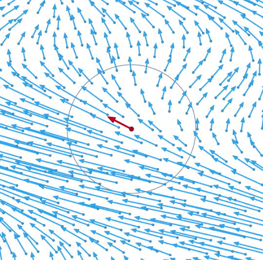
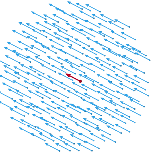
The antisymmetric term R represents a rigid-like rotation of the fluid about the point p. Its angular velocity ω is

[math]\displaystyle{ \omega=\tfrac12 \nabla\times \mathbf{v}= \tfrac12 \begin{bmatrix} \partial_2 v_3-\partial_3 v_2\\ \partial_3 v_1-\partial_1 v_3\\ \partial_1 v_2-\partial_2 v_1 \end{bmatrix}. }[/math]

The product ∇ × v is called the rotational curl of the vector field. A rigid rotation does not change the relative positions of the fluid elements, so the antisymmetric term R of the velocity gradient does not contribute to the rate of change of the deformation. The actual strain rate is therefore described by the symmetric E term, which is the strain rate tensor.

1.2. Shear Rate and Compression Rate

The scalar part D(p,t)(r) (uniform expansion/compression rate) of the strain rate tensor E(p,t)(r). https://handwiki.org/wiki/index.php?curid=1553684

The traceless part S(p,t)(r) (shear rate) of the strain rate tensor E(p,t)(r). https://handwiki.org/wiki/index.php?curid=1803999

The symmetric term E of velocity gradient (the rate-of-strain tensor) can be broken down further as the sum of a scalar times the unit tensor, that represents a gradual isotropic expansion or contraction; and a traceless symmetric tensor which represents a gradual shearing deformation, with no change in volume:^[1]

[math]\displaystyle{ \mathbf{E}(\mathbf{p},t)(\mathbf{r}) = \mathbf{D}(\mathbf{p},t)(\mathbf{r}) + \mathbf{S}(\mathbf{p},t)(\mathbf{r}). }[/math]

That is,

[math]\displaystyle{ E_{ij} = \underbrace{\tfrac13\left(\sum_k\partial_k v_k\right) \delta_{ij}}_{\text{rate-of-expansion tensor} D_{ij}} + \underbrace{\tfrac12\left(\partial_i v_j+\partial_j v_i\right)-\tfrac13\left(\sum_k\partial_k v_k\right) \delta_{ij}}_{\text{rate-of-shear tensor} S_{ij}}, }[/math]

Here δ is the unit tensor, such that δ_ij is 1 if i = j and 0 if i ≠ j. This decomposition is independent of the choice of coordinate system, and is therefore physically significant.

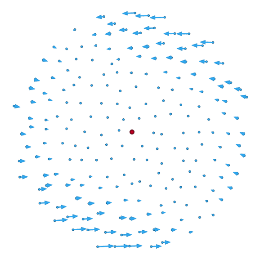
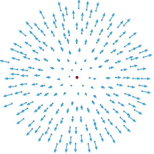
The expansion rate tensor is 1/3 of the divergence of the velocity field:

[math]\displaystyle{ \nabla \cdot \mathbf{v} = \partial_1 v_1 + \partial_2 v_2 + \partial_3 v_3; }[/math]

which is the rate at which the volume of a fixed amount of fluid increases at that point.

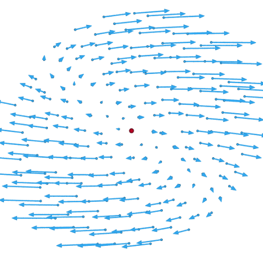
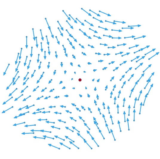
The shear rate tensor is represented by a symmetric 3 × 3 matrix, and describes a flow that combines compression and expansion flows along three orthogonal axes, such that there is no change in volume. This type of flow occurs, for example, when a rubber strip is stretched by pulling at the ends, or when honey falls from a spoon as a smooth unbroken stream.

For a two-dimensional flow, the divergence of v has only two terms and quantifies the change in area rather than volume. The factor 1/3 in the expansion rate term should be replaced by 1/2 in that case.

References

- Landau, L. D.; Lifshitz, E. M. (1997). Fluid Mechanics (2nd ed.). Butterworth Heinemann. ISBN 0-7506-2767-0.