1. Overview

Given a signal of interest ${\displaystyle \mathbf{x}\in {\mathbb{R}}^N}$ and a redundant dictionary ${\displaystyle \mathbf{D}\in {\mathbb{R}}^{N\times M},M\gg N}$, the Sparse Coding problem consist of retrieving a sparse vector ${\displaystyle \mathbf{\Gamma }\in {\mathbb{R}}^M}$, denominated the Sparse representation of ${\displaystyle \mathbf{x}}$, such that ${\displaystyle \mathbf{x}=\mathbf{D}\mathbf{\Gamma }}$. Intuitively, this implies ${\displaystyle \mathbf{x}}$ is expressed as a linear combination of a small number of elements in ${\displaystyle \mathbf{D}}$. The global sparsity constraint prior has been shown to be useful in many ill-posed inverse problems such as image inpainting, super-resolution, and coding.^[1][2][3] It has been of particular interest for image understanding and computer vision tasks involving natural images, allowing redundant dictionaries to be efficiently inferred ^[4][5][6]

As an extension to the global sparsity constraint, recent pieces in the literature have revisited the model to reach a more profound understanding of its uniqueness and stability conditions.^[6] Interestingly, by imposing a local sparsity prior in ${\displaystyle \mathbf{\Gamma }}$, meaning that its independent patches can be interpreted as sparse vectors themselves, the structure in ${\displaystyle \mathbf{D}}$ can be understood as a “local" dictionary operating over each independent patch. This model extension is denominated Convolutional Sparse Coding (CSC) and drastically reduces the burden of estimating signal representations while being characterized by stronger uniqueness and stability conditions. Furthermore, it allows for ${\displaystyle \mathbf{\Gamma }}$ to be efficiently estimated via projected gradient descent algorithms such as Orthonormal Matching Pursuit and Basis Pursuit, while performing in a local fashion^[5]

Besides its versatility in inverse problems, recent efforts have focused on the multi-layer version of the model and provided evidence of its reliability for recovering multiple underlying representations.^[7] Moreover, a tight connection between such a model and the well-established Convolutional Neural Network model (CNN) was revealed, providing a new tool for a more rigurous understanding of its theoretical conditions.

The convolutional sparse coding model provides a very efficient set of tools to solve a wide range of inverse problems, including image denoising, image inpainting, and image superresolution. By imposing local sparsity constraints, it allows to efficiently tackle the global coding problem by iteratively estimating disjoint patches and assembling them into a global signal. Furthermore, by adopting a multi-layer sparse model, which results from imposing the sparsity constraint to the signal inherent representations themselves, the resulting “Layered" Pursuit algorithm keeps the strong uniqueness and stability conditions from the single-layer model. This extension also provides some interesting notions about the relation between its sparsity prior and the forward pass of the Convolutional Neural Network, which allows to understand how the theoretical benefits of the CSC model can provide a strong mathematical meaning of the CNN structure.

2. Sparse Coding Paradigm

Basic concepts and models are presented to explain into detail the Convolutional Sparse Representation framework. On the grounds that the sparsity constraint has been proposed under different models, a short description of them is presented to show its evolution up to the model of interest. Also included are the concepts of Mutual Coherence and Restricted Isometry Property to establish uniqueness stability guarantees.

2.1. Global Sparse Coding Model

Allow signal ${\displaystyle \mathbf{x}\in {\mathbb{R}}^N}$ to be expressed as a linear combination of a small number of atoms from a given dictionary ${\displaystyle \mathbf{D}\in {\mathbb{R}}^{N\times M},M>N}$. Alternatively, the signal can be expressed as ${\displaystyle \mathbf{x}=\mathbf{D}\mathbf{\Gamma }}$, where ${\displaystyle \mathbf{\Gamma }\in {\mathbb{R}}^M}$ corresponds to the sparse representation of ${\displaystyle \mathbf{x}}$, which selects the atoms to combine and their weights. Subsequently, given ${\displaystyle \mathbf{D}}$, the task of recovering ${\displaystyle \mathbf{\Gamma }}$ from either the noise-free signal itself or an observation is denominated sparse coding. Considering the noise-free scenario, the coding problem is formulated as follows: $\text{Unknown environment 'aligned'}$ The effect of the ${\displaystyle {\ell }_0}$ norm is to favor solutions with as much zero elements as possible. Furthermore, given an observation affected by bounded energy noise: ${\displaystyle \mathbf{Y}=\mathbf{D}\mathbf{\Gamma }+\mathbf{E},\Vert \mathbf{E}{\Vert }_2<\epsilon }$, the pursuit problem is reformulated as: $\text{Unknown environment 'aligned'}$

2.2. Stability and Uniqueness Guarantees for the Global Sparse Model

Let the spark of ${\displaystyle \mathbf{D}}$ be defined as the minimum number of linearly independent columns: $\text{Unknown environment 'aligned'}$

Then, from the triangular inequality, the sparsest vector ${\displaystyle \mathbf{\Gamma }}$ satisfies: ${\displaystyle \Vert \mathbf{\Gamma }{\Vert }_0<\frac{\sigma (\mathbf{D})}{2}}$. Although the spark provides an upper bound, it is unfeasible to compute in practical scenarios. Instead, let the mutual coherence be a measure of similarity between atoms in ${\displaystyle \mathbf{D}}$. Assuming ${\displaystyle {\ell }_2}$-norm unit atoms, the mutual coherence of ${\displaystyle \mathbf{D}}$ is defined as: ${\displaystyle \mu (\mathbf{D})=\underset{i\ne j}{max}\Vert {\mathbf{d}}_{\mathbf{i}}^{\mathbf{T}}{\mathbf{d}}_{\mathbf{j}}{\Vert }_2}$, where ${\displaystyle {\mathbf{d}}_i}$ are atoms. Based on this metric, it can be proven that the true sparse representation ${\displaystyle {\mathbf{\Gamma }}^{\ast }}$ can be recovered if and only if ${\displaystyle \Vert {\mathbf{\Gamma }}^{\ast }{\Vert }_0<\frac{1}{2}(1+\frac{1}{\mu (\mathbf{D})})}$.

Similarly, under the presence of noise, an upper bound for the distance between the true sparse representation ${\displaystyle {\mathbf{\Gamma }}^{\mathbf{\ast }}}$ and its estimation ${\displaystyle \hat{\mathbf{\Gamma }}}$ can be established via the Restricted Isometry Property (RIP). A k-RIP matrix ${\displaystyle \mathbf{D}}$ with constant ${\displaystyle {\delta }_k}$ corresponds to: ${\displaystyle (1-{\delta }_k)\Vert \mathbf{\Gamma }{\Vert }_2^2\le \Vert \mathbf{D}\mathbf{\Gamma }{\Vert }_2^2\le (1+{\delta }_k)\Vert \mathbf{\Gamma }{\Vert }_2^2}$, where ${\displaystyle {\delta }_k}$ is the smallest number that satisfies the inequality for every ${\displaystyle \Vert \mathbf{\Gamma }{\Vert }_0=k}$. Then, assuming ${\displaystyle \Vert \mathbf{\Gamma }{\Vert }_0<\frac{1}{2}(1+\frac{1}{\mu (\mathbf{D})})}$, it is guaranteed that ${\displaystyle \Vert \hat{\mathbf{\Gamma }}\mathbf{-}{\mathbf{\Gamma }}^{\mathbf{\ast }}{\Vert }_2^2\le \frac{4{\epsilon }^2}{1-\mu (\mathbf{D})(2\Vert \mathbf{\Gamma }{\Vert }_0-1)}}$.

Solving such a general pursuit problem is a hard task if no structure is imposed on dictionary ${\displaystyle \mathbf{D}}$. This implies learning large, highly overcomplete representations, which is extremely expensive. Assuming such a burden has been met and a representative dictionary has been obtained for a given signal ${\displaystyle \mathbf{x}}$, typically based on prior information, ${\displaystyle {\mathbf{\Gamma }}^{\ast }}$ can be estimated via several pursuit algorithms.

Pursuit algorithms for the global sparse model

Two basic methods for solving the Global Sparse Coding problem are Orthogonal Matching Pursuit (OMP) and Basis Pursuit (BP) . OMP is a greedy algorithm that iteratively selects the atom best correlated with the residual between ${\displaystyle \mathbf{x}}$ and a current estimation, followed by a projection onto a subset of pre-selected atoms. On the other hand, BP is a more sophisticated approach that replaces the original coding problem by a linear programming problem. Based on this algorithms, the Global Sparse Coding provides considerably loose bounds for the uniqueness and stability of ${\displaystyle \hat{\mathbf{\Gamma }}}$. To overcome this, additional priors are imposed over ${\displaystyle \mathbf{D}}$ to guarantee tighter bounds and uniqueness conditions. The reader is referred to (,^[5] section 2) for details regarding this properties.

2.3. Convolutional Sparse Coding Model

A local prior is adopted such that each overlapping section of ${\displaystyle \mathbf{\Gamma }}$ is sparse. Let ${\displaystyle \mathbf{D}\in {\mathbb{R}}^{N\times Nm}}$ be constructed from shifted versions of a local dictionary ${\displaystyle {\mathbf{D}}_{\mathbf{L}}\in {\mathbb{R}}^{n\times m},m\ll M}$. Then, ${\displaystyle \mathbf{x}}$ is formed by products between ${\displaystyle {\mathbf{D}}_{\mathbf{L}}}$ and local patches of ${\displaystyle \mathbf{\Gamma }\in {\mathbb{R}}^{mN}}$.

The global dictionary is expressed in terms of a stride convolutional matrix. So, signals can be generated in terms of stripes of the sparse representation multiplies by a shift-invariant local dictionary. https://handwiki.org/wiki/index.php?curid=2065104

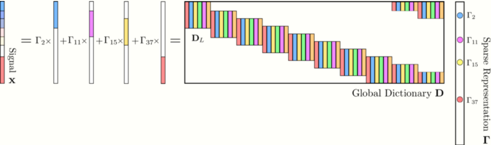
From the latter, ${\displaystyle \mathbf{\Gamma }}$ can be re-expressed by ${\displaystyle N}$ disjoint sparse vectors ${\displaystyle {\alpha }_i\in {\mathbb{R}}^m}$: ${\displaystyle \mathbf{\Gamma }\in \{{\alpha }_1,{\alpha }_2,\dots ,{\alpha }_N{\}}^T}$. Similarly, let ${\displaystyle \gamma }$ be a set of ${\displaystyle (2n-1)}$ consecutive vectors ${\displaystyle {\alpha }_i}$. Then, each disjoint segment in ${\displaystyle \mathbf{x}}$ is expressed as: ${\displaystyle {\mathbf{x}}_i={\mathbf{R}}_i\mathbf{D}\mathbf{\Gamma }}$, where operator ${\displaystyle {\mathbf{R}}_i\in {\mathbb{R}}^{n\times N}}$ extracts overlapping patches of size ${\displaystyle n}$ starting at index ${\displaystyle i}$. Thus, ${\displaystyle {\mathbf{R}}_i\mathbf{D}}$ contains only ${\displaystyle (2n-1)m}$ nonzero columns. Hence, by introducing operator ${\displaystyle {\mathbf{S}}_i\in {\mathbf{R}}^{(2n-1)m\times Nm}}$ which exclusively preserves them: $\text{Unknown environment 'aligned'}$ where ${\displaystyle \mathrm{\Omega }}$ is known as the stripe dictionary, which is independent of ${\displaystyle i}$, and ${\displaystyle {\gamma }_i}$ is denominated the i-th stripe. So, ${\displaystyle \mathbf{x}}$ corresponds to a patch aggregation or convolutional interpretation: $\text{Unknown environment 'aligned'}$ Where ${\displaystyle {\mathbf{d}}_i}$ corresponds to the i-th atom from the local dictionary ${\displaystyle {\mathbf{D}}_L}$ and ${\displaystyle {\mathbf{z}}_{\mathbf{i}}}$ is constructed by elements of patches ${\displaystyle \alpha }$: $\text{Undefined control sequence triangleq}$. Given the new dictionary structure, let the ${\displaystyle {\ell }_{0,\mathrm{\infty }}}$ pseudo-norm be defined as: $\text{Undefined control sequence triangleq}$. Then, for the noise-free and noise-corrupted scenarios, the problem can be respectively reformulated as: $\text{Unknown environment 'aligned'}$

Stability and uniqueness guarantees for the convolutional sparse model

For the local approach, ${\displaystyle \mathbf{D}}$ mutual coherence satisfies: ${\displaystyle \mu (\mathbf{D})\ge (\frac{m-1}{m(2n-1)-1}{)}^{1/2}.}$ So, if a solution obeys ${\displaystyle \Vert \mathbf{\Gamma }{\Vert }_{0,\mathrm{\infty }}<\frac{1}{2}(1+\frac{1}{\mu (\mathbf{D})})}$, then it is the sparsest solution to the ${\displaystyle {\ell }_{0,\mathrm{\infty }}}$ problem. Thus, under the local formulation, the same number of non-zeros is permitted for each stripe instead of the full vector!

Similar to the global model, the CSC is solved via OMP and BP methods, the latter contemplating the use of the Iterative Shrinkage Thresholding Algorithm (ISTA)^[8] for splitting the pursuit into smaller problems. Based on the ${\displaystyle {\ell }_{0,\mathrm{\infty }}}$ pseudonorm, if a solution ${\displaystyle \mathbf{\Gamma }}$ exists satisfying ${\displaystyle \Vert \mathbf{\Gamma }{\Vert }_{0,\mathrm{\infty }}<\frac{1}{2}(1+\frac{1}{\mu (\mathbf{D})})}$, then both methods are guaranteed to recover it. Moreover, the local model guarantees recovery independently of the signal dimension, as opposed to the ${\displaystyle {\ell }_0}$ prior. Stability conditions for OMP and BP are also guaranteed if its Exact Recovery Condition (ERC) is met for a support ${\displaystyle \mathcal{T}}$ with a constant ${\displaystyle \theta }$. The ERC is defined as: ${\displaystyle \theta =1-\underset{i\notin \mathcal{T}}{\text{max}}\Vert {\mathbf{D}}_{\mathcal{T}}^{†}{\mathbf{d}}_i{\Vert }_1>0}$, where ${\displaystyle †}$ denotes the Pseudo-inverse. Algorithm 1 shows the Global Pursuit method based on ISTA.

Algorithm 1: 1D CSC via local iterative soft-thresholding.

Input:

${\displaystyle {\mathbf{D}}_L}$: Local Dictionary,

${\displaystyle \mathbf{y}}$: observation,

${\displaystyle \lambda }$: Regularization parameter,

${\displaystyle c}$: step size for ISTA,

tol: tolerance factor,

maxiters: maximum number of iterations.

$\text{Undefined control sequence boldsymbol}$ (Initialize disjoint patches.)

${\displaystyle \{{\mathbf{r}}_i{\}}^{(0)}\leftarrow \{{\mathbf{R}}_i\mathbf{y}\}}$ (Initialize residual patches.)

${\displaystyle k\leftarrow 0}$

Repeat

$\text{Undefined control sequence boldsymbol}$ (Coding along disjoint patches)

$\text{Undefined control sequence boldsymbol}$ $\text{Undefined control sequence boldsymbol}$ (Patch Aggregation)

${\displaystyle \{{\mathbf{r}}_i{\}}^{(k)}\leftarrow {\mathbf{R}}_i(\mathbf{y}-{\hat{\mathbf{x}}}^{(k)})}$ (Update residuals)

${\displaystyle k\leftarrow k+1}$

Until ${\displaystyle \Vert {\hat{\mathbf{x}}}^{(k)}-{\hat{\mathbf{x}}}^{(k-1)}{\Vert }_2<}$ tol or ${\displaystyle k>}$ maxiters.

2.4. Multi-Layered Convolutional Sparse Coding Model

By imposing the sparsity prior in the inherent structure of ${\displaystyle \mathbf{x}}$, strong conditions for a unique representation and feasible methods for estimating it are granted. Similarly, such a constraint can be applied to its representation itself, generating a cascade of sparse representations: Each code is defined by a few atoms of a given set of convolutional dictionaries.

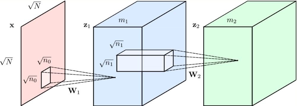
Based on this criteria, yet another extension denominated Multi-layer Convolutional Sparse Coding (ML-CSC) is proposed. A set of analytical dictionaries ${\displaystyle \{\mathbf{D}{\}}_{k=1}^K}$ can be efficiently designed, where sparse representations at each layer ${\displaystyle \{\mathbf{\Gamma }{\}}_{k=1}^K}$ are guaranteed by imposing the sparsity prior over the dictionaries themselves.^[7] In other words, by considering dictionaries to be stride convolutional matrices i.e. atoms of the local dictionaries shift ${\displaystyle m}$ elements instead of a single one, where ${\displaystyle m}$ corresponds to the number of channels in the previous layer, it is guaranteed that the ${\displaystyle \Vert \mathbf{\Gamma }{\Vert }_{0,\mathrm{\infty }}}$ norm of the representations along layers is bounded.

For example, given the dictionaries ${\displaystyle {\mathbf{D}}_1\in {\mathbb{R}}^{N\times N{m}_1},{\mathbf{D}}_2\in {\mathbb{R}}^{N{m}_1\times N{m}_2}}$, the signal is modeled as ${\displaystyle {\mathbf{D}}_1{\mathbf{\Gamma }}_1={\mathbf{D}}_1({\mathbf{D}}_2{\mathbf{\Gamma }}_2)}$, where ${\displaystyle {\mathbf{\Gamma }}_1}$ is its sparse code, and ${\displaystyle {\mathbf{\Gamma }}_2}$ is the sparse code of ${\displaystyle {\mathbf{\Gamma }}_1}$. Then, the estimation of each representation is formulated as an optimization problem for both noise-free and noise-corrupted scenarios, respectively. Assuming ${\displaystyle {\mathbf{\Gamma }}_0=\mathbf{x}}$: $\text{Unknown environment 'aligned'}$

In what follows, theoretical guarantees for the uniqueness and stability of this extended model are described.

Theorem 1: (Uniqueness of Sparse Representations) Consider signal ${\displaystyle \mathbf{x}}$ satisfies the (ML-CSC) model for a set of convolutional dictionaries ${\displaystyle \{{\mathbf{D}}_i{\}}_{i=1}^K}$ with mutual coherence ${\displaystyle \{\mu ({\mathbf{D}}_i){\}}_{i=1}^K}$. If the true sparse representations satisfy ${\displaystyle \{\mathbf{\Gamma }{\}}_{i=1}^K<\frac{1}{2}(1+\frac{1}{\mu ({\mathbf{D}}_i)})}$, then a solution to the problem ${\displaystyle \{\widehat{{\mathbf{\Gamma }}_i}{\}}_{i=1}^K}$ will be its unique solution if the thresholds are chosen to satisfy: ${\displaystyle {\lambda }_i<\frac{1}{2}(1+\frac{1}{\mu ({\mathbf{D}}_i)})}$.

Theorem 2: (Global Stability of the noise-corrupted scenario) Consider signal ${\displaystyle \mathbf{x}}$ satisfies the (ML-CSC) model for a set of convolutional dictionaries ${\displaystyle \{{\mathbf{D}}_i{\}}_{i=1}^K}$ is contaminated with noise ${\displaystyle \mathbf{E}}$, where ${\displaystyle \Vert \mathbf{E}{\Vert }_2\le {\epsilon }_0}$. resulting in ${\displaystyle \mathbf{Y}\mathbf{=}\mathbf{X}\mathbf{+}\mathbf{E}}$. If ${\displaystyle {\lambda }_i<\frac{1}{2}(1+\frac{1}{\mu ({\mathbf{D}}_i)})}$ and ${\displaystyle {\epsilon }_i^2=\frac{4{\epsilon }_{i-1}^2}{1-(2\Vert {\mathbf{\Gamma }}_i{\Vert }_{0,\mathrm{\infty }}-1)\mu ({\mathbf{D}}_i)}}$, then the estimated representations ${\displaystyle \{{\mathbf{\Gamma }}_i{\}}_{i=1}^K}$ satisfy the following: ${\displaystyle \Vert {\mathbf{\Gamma }}_i-{\hat{\mathbf{\Gamma }}}_i{\Vert }_2^2\le {\epsilon }_i^2}$.

2.5. Projection-Based Algorithms

As a simple approach for solving the ML-CSC problem, either via the ${\displaystyle {\ell }_0}$ or ${\displaystyle {\ell }_1}$ norms, is by computing inner products between ${\displaystyle \mathbf{x}}$ and the dictionary atoms to identify the most representatives ones. Such a projection is described as: $\text{Unknown environment 'aligned'}$

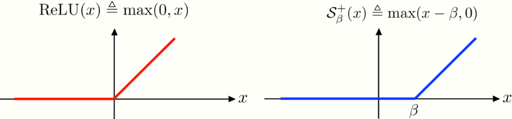
which have closed-form solutions via the hard-thresholding ${\displaystyle {\mathcal{H}}_{\beta }({\mathbf{D}}^T\mathbf{x})}$ and soft-thresholding algorithms ${\displaystyle {\mathcal{S}}_{\beta }({\mathbf{D}}^T\mathbf{x})}$, respectively. If a nonnegative constraint is also contemplated, the problem can be expressed via the ${\displaystyle {\ell }_1}$ norm as: $\text{Unknown environment 'aligned'}$ which closed-form solution corresponds to the soft nonnegative thresholding operator ${\displaystyle {\mathcal{S}}_{\beta }^{+}({\mathbf{D}}^T\mathbf{x})}$, where $\text{Undefined control sequence triangleq}$. Guarantees for the Layered soft-thresholding approach are included in the Appendix (Section 6.2).

Theorem 3: (Stable recovery of the multi-layered soft-thresholding algorithm) Consider signal ${\displaystyle \mathbf{x}}$ that satisfies the (ML-CSC) model for a set of convolutional dictionaries ${\displaystyle \{{\mathbf{D}}_i{\}}_{i=1}^K}$ with mutual coherence ${\displaystyle \{\mu ({\mathbf{D}}_i){\}}_{i=1}^K}$ is contaminated with noise ${\displaystyle \mathbf{E}}$, where ${\displaystyle \Vert \mathbf{E}{\Vert }_2\le {\epsilon }_0}$. resulting in ${\displaystyle \mathbf{Y}\mathbf{=}\mathbf{X}\mathbf{+}\mathbf{E}}$. Denote by ${\displaystyle |{\mathbf{\Gamma }}_i^{min}|}$ and ${\displaystyle |{\mathbf{\Gamma }}_i^{max}|}$ the lowest and highest entries in ${\displaystyle {\mathbf{\Gamma }}_i}$. Let ${\displaystyle \{{\hat{\mathbf{\Gamma }}}_i{\}}_{i=1}^K}$ be the estimated sparse representations obtained for ${\displaystyle \{{\beta }_i{\}}_{i=1}^K}$. If ${\displaystyle \Vert {\mathbf{\Gamma }}_i{\Vert }_{0,\mathrm{\infty }}<\frac{1}{2}(1+\frac{1}{\mu ({\mathbf{D}}_i)}\frac{|{\mathbf{\Gamma }}_i^{min}|}{|{\mathbf{\Gamma }}_i^{min}|})-\frac{1}{\mu ({\mathbf{D}}_i)}\frac{{\epsilon }_{i-1}}{|{\mathbf{\Gamma }}_i^{max}|}}$ and ${\displaystyle {\beta }_i}$ is chosen according to: $\text{Unknown environment 'aligned'}$ Then, ${\displaystyle {\hat{\mathbf{\Gamma }}}_i}$ has the same support as ${\displaystyle {\mathbf{\Gamma }}_i}$, and ${\displaystyle \Vert {\mathbf{\Gamma }}_i-\widehat{{\mathbf{\Gamma }}_i}{\Vert }_{2,\mathrm{\infty }}\le {\epsilon }_i}$, for ${\displaystyle {\epsilon }_i=\sqrt{\Vert {\mathbf{\Gamma }}_i{\Vert }_{0,\mathrm{\infty }}}({\epsilon }_{i-1}+\mu ({\mathbf{D}}_i)(\Vert {\mathbf{\Gamma }}_i{\Vert }_{0,\mathrm{\infty }}-1)|{\mathbf{\Gamma }}_i^{max}|+{\beta }_i)}$

2.6. Connections to Convolutional Neural Networks

Recall the Forward Pass of the Convolutional Neural Network (CNN) model, used in both training and inference steps. Let ${\displaystyle \mathbf{x}\in {\mathbb{R}}^{M{m}_1}}$ be its input and ${\displaystyle {\mathbf{W}}_k\in {\mathbb{R}}^{N\times m_1}}$ the filters at layer ${\displaystyle k}$, which are followed by the Rectified Linear Unit ${\displaystyle \text{ReLU}(\mathbf{x})=max(0,x)}$, for bias ${\displaystyle \mathbf{b}\in {\mathbb{R}}^{M{m}_1}}$. Based on this elementary block, taking ${\displaystyle K=2}$ as example, the CNN output can be expressed as: $\text{Unknown environment 'aligned'}$ Finally, comparing the CNN algorithm and the Layered thresholding approach for the nonnegative constaint [sic?], it is straightforward to show that both are equivalent: $\text{Unknown environment 'aligned'}$

Convolutional Layers from the Forward Pass Algorithm. https://handwiki.org/wiki/index.php?curid=2057193

Contrast between the rectified linear unit function and the nonnegative soft thresholding pointwise nonlinearities. https://handwiki.org/wiki/index.php?curid=2082172

As explained in what follows, this naive approach of solving the coding problem is a particular case of a more stable projected gradient descent algorithm for the ML-CSC model. Equipped with the stability conditions of both approaches, a more clear understanding about the class of signals a CNN can recover, under what noise conditions can an estimation be accurately attained, and how can its structure be modified to improve its theoretical conditions. The reader is referred to (,^[7] section 5) for details regarding their connection.

2.7. Pursuit Algorithms for the Multi-Layer CSC Model

A crucial limitation of the Forward Pass is it being unable to recover the unique solution of the DCP problem, which existence has been demonstrated. So, instead of using a thresholding approach at each layer, a full pursuit method is adopted, denominated Layered Basis Pursuit (LBP). Considering the projection onto the ${\displaystyle {\ell }_1}$ ball, the following problem is proposed: $\text{Unknown environment 'aligned'}$ where each layer is solved as an independent CSC problem, and ${\displaystyle {\xi }_i}$ is proportional to the noise level at each layer. Among the methods for solving the layered coding problem, ISTA is an efficient decoupling alternative. In what follows, a short summary of the guarantees for the LBP are established.

Theorem 4: (Recovery guarantee) Consider a signal ${\displaystyle \mathbf{x}}$ characterized by a set of sparse vectors ${\displaystyle \{{\mathbf{\Gamma }}_i{\}}_{i=1}^K}$, convolutional dictionaries ${\displaystyle \{{\mathbf{D}}_i{\}}_{i=1}^K}$ and their corresponding mutual coherences ${\displaystyle \{\mu ({\mathbf{D}}_i){\}}_{i=1}^K}$. If ${\displaystyle \Vert {\mathbf{\Gamma }}_i{\Vert }_{0,\mathrm{\infty }}<\frac{1}{2}(1+\frac{1}{\mu ({\mathbf{D}}_i)})}$, then the LBP algorithm is guaranteed to recover the sparse representations.

Theorem 5: (Stability in the presence of noise) Consider the contaminated signal ${\displaystyle \mathbf{Y}=\mathbf{X}\mathbf{+}\mathbf{E}}$, where ${\displaystyle \Vert \mathbf{E}{\Vert }_{0,\mathrm{\infty }}\le {\epsilon }_0}$ and ${\displaystyle \mathbf{x}}$ is characterized by a set of sparse vectors ${\displaystyle \{{\mathbf{\Gamma }}_i{\}}_{i=1}^K}$ and convolutional dictionaries ${\displaystyle \{{\mathbf{D}}_i{\}}_{i=1}^K}$. Let ${\displaystyle \{{\hat{\mathbf{\Gamma }}}_i{\}}_{i=1}^K}$ be solutions obtained via the LBP algorithm with parameters ${\displaystyle \{\xi {\}}_{i=1}^K}$. If ${\displaystyle \Vert {\mathbf{\Gamma }}_i{\Vert }_{0,\mathrm{\infty }}<\frac{1}{3}(1+\frac{1}{\mu ({\mathbf{D}}_i)})}$ and ${\displaystyle {\xi }_i=4{\epsilon }_{i-1}}$, then: (i) The support of the solution ${\displaystyle {\hat{\mathbf{\Gamma }}}_i}$ is contained in that of ${\displaystyle {\mathbf{\Gamma }}_i}$, (ii) $\text{Missing argument for mathbf}$, and (iii) Any entry greater in absolute value than ${\displaystyle \frac{{\epsilon }_i}{\sqrt{\Vert {\mathbf{\Gamma }}_i{\Vert }_{0\mathrm{\infty }}}}}$ is guaranteed to be recovered.

3. Applications of the Convolutional Sparse Coding Model: Image Inpainting

As a practical example, an efficient image inpainting method for color images via the CSC model is shown.^[6] Consider the three-channel dictionary ${\displaystyle \mathbf{D}\in {\mathbb{R}}^{N\times M\times 3}}$, where ${\displaystyle {\mathbf{d}}_{c,m}}$ denotes the ${\displaystyle m}$-th atom at channel ${\displaystyle c}$, represents signal ${\displaystyle \mathbf{x}}$ by a single cross-channel sparse representation ${\displaystyle \mathbf{\Gamma }}$, with stripes denoted as ${\displaystyle {\mathbf{z}}_i}$. Given an observation ${\displaystyle \mathbf{y}=\{{\mathbf{y}}_r,{\mathbf{y}}_g,{\mathbf{y}}_b\}}$, where randomly chosen channels at unknown pixel locations are fixed to zero, in a similar way to impulse noise, the problem is formulated as: $\text{Unknown environment 'aligned'}$ By means of ADMM,^[9] the cost function is decoupled into simpler sub-problems, allowing an efficient ${\displaystyle \mathbf{\Gamma }}$ estimation. Algorithm 2 describes the procedure, where ${\displaystyle {\hat{D}}_{c,m}}$ is the DFT representation of ${\displaystyle D_{c,m}}$, the convolutional matrix for the term ${\displaystyle {\mathbf{d}}_{c,i}\ast {\mathbf{z}}_i}$. Likewise, ${\displaystyle {\hat{\mathbf{x}}}_m}$ and ${\displaystyle {\hat{\mathbf{z}}}_m}$ correspond to the DFT representations of ${\displaystyle {\mathbf{x}}_m}$ and ${\displaystyle {\mathbf{z}}_m}$, respectively, ${\displaystyle {\mathcal{S}}_{\beta }(.)}$ corresponds to the Soft-thresholding function with argument ${\displaystyle \beta }$, and the ${\displaystyle {\ell }_{1,2}}$ norm is defined as the ${\displaystyle {\ell }_2}$ norm along the channel dimension ${\displaystyle c}$ followed by the ${\displaystyle {\ell }_1}$ norm along the spatial dimension ${\displaystyle m}$. The reader is referred to (,^[6] Section II) for details on the ADMM implementation and the dictionary learning procedure.

Algorithm 2: Color image inpainting via the convolutional sparse coding model.

Input:

${\displaystyle {\hat{\mathbf{D}}}_{c,m}}$: DFT of convolutional matrices ${\displaystyle {\mathbf{D}}_{c,m}}$,

${\displaystyle \mathbf{y}=\{{\mathbf{y}}_r,{\mathbf{y}}_g,{\mathbf{y}}_b\}}$: Color observation,

${\displaystyle \lambda }$: Regularization parameter,

${\displaystyle \{\mu ,\rho \}}$: step sizes for ADMM,

tol: tolerance factor,

maxiters: maximum number of iterations.

${\displaystyle k\leftarrow k+1}$

Repeat

${\displaystyle \{{\hat{\mathbf{z}}}_m{\}}^{(k+1)}\leftarrow \underset{\{{\hat{\mathbf{x}}}_m\}}{\text{argmin}}\frac{1}{2}\sum _c\Vert \sum _m{\hat{\mathbf{D}}}_{c,m}{\hat{\mathbf{z}}}_m-{\hat{\mathbf{y}}}_c\Vert +\frac{\rho }{2}\sum _m\Vert {\hat{\mathbf{z}}}_m-({\hat{\mathbf{y}}}_m+{\hat{\mathbf{u}}}_m^{(k)}){\Vert }_2^2.}$

${\displaystyle \{{\mathbf{y}}_{c,m}{\}}^{(k+1)}\leftarrow \underset{\{{\mathbf{y}}_{c,m}\}}{\text{argmin}}\lambda \sum _c\sum _m\Vert {\mathbf{y}}_{c,m}{\Vert }_1+\mu \Vert \{{\mathbf{x}}_{c,m}^{(k+1)}\}{\Vert }_{2,1}+\frac{\rho }{2}\sum _m\Vert {\mathbf{z}}_m^{(k+1)}-(\mathbf{y}+{\mathbf{u}}_m^{(k)}){\Vert }_2^2.}$

${\displaystyle {\mathbf{y}}_m^{(k+1)}={\mathcal{S}}_{\lambda /\rho }({\mathbf{x}}_m^{(k+1)}+{\mathbf{u}}_m^{(k)}).}$

${\displaystyle k\leftarrow k+1}$

Until ${\displaystyle \Vert \{{\mathbf{z}}_m{\}}^{(k+1)}-\{{\mathbf{z}}_m{\}}^{(k)}{\Vert }_2<}$tol or ${\displaystyle i>}$ maxiters.

References

- Jianchao Yang; Wright, John; Huang, Thomas S; Yi Ma (November 2010). "Image Super-Resolution Via Sparse Representation". IEEE Transactions on Image Processing 19 (11): 2861–2873. doi:10.1109/TIP.2010.2050625. PMID 20483687. Bibcode: 2010ITIP...19.2861Y. https://dx.doi.org/10.1109%2FTIP.2010.2050625
- Wetzstein, Gordon; Heidrich, Wolfgang; Heide, Felix (2015). Fast and Flexible Convolutional Sparse Coding. pp. 5135–5143. https://www.cv-foundation.org/openaccess/content_cvpr_2015/html/Heide_Fast_and_Flexible_2015_CVPR_paper.html.
- Wohlberg, Brendt (2017). "SPORCO: A Python package for standard and convolutional sparse representations". Proceedings of the 16th Python in Science Conference: 1–8. doi:10.25080/shinma-7f4c6e7-001. http://conference.scipy.org/proceedings/scipy2017/brendt_wohlberg.html.
- Mairal, Julien; Bach, Francis; Ponce, Jean; Sapiro, Guillermo (2009). "Online Dictionary Learning for Sparse Coding". Proceedings of the 26th Annual International Conference on Machine Learning (ACM): 689–696. doi:10.1145/1553374.1553463. ISBN 9781605585161. https://dl.acm.org/citation.cfm?id=1553463.
- Papyan, Vardan; Sulam, Jeremias; Elad, Michael (1 November 2017). "Working Locally Thinking Globally: Theoretical Guarantees for Convolutional Sparse Coding". IEEE Transactions on Signal Processing 65 (21): 5687–5701. doi:10.1109/TSP.2017.2733447. Bibcode: 2017ITSP...65.5687P. https://dx.doi.org/10.1109%2FTSP.2017.2733447
- Wohlberg, Brendt (6–8 March 2016). "Convolutional sparse representation of color images". 2016 IEEE Southwest Symposium on Image Analysis and Interpretation (SSIAI): 57–60. doi:10.1109/SSIAI.2016.7459174. ISBN 978-1-4673-9919-7. https://dx.doi.org/10.1109%2FSSIAI.2016.7459174
- Papyan, Vardan; Romano, Yaniv; Elad, Michael (2017). "Convolutional Neural Networks Analyzed via Convolutional Sparse Coding". J. Mach. Learn. Res. 18 (1): 2887–2938. ISSN 1532-4435. Bibcode: 2016arXiv160708194P. http://dl.acm.org/citation.cfm?id=3122009.3176827.
- Beck, Amir; Teboulle, Marc (January 2009). "A Fast Iterative Shrinkage-Thresholding Algorithm for Linear Inverse Problems". SIAM Journal on Imaging Sciences 2 (1): 183–202. doi:10.1137/080716542. https://dx.doi.org/10.1137%2F080716542
- Boyd, Stephen (2010). "Distributed Optimization and Statistical Learning via the Alternating Direction Method of Multipliers". Foundations and Trends in Machine Learning 3 (1): 1–122. doi:10.1561/2200000016. ISSN 1935-8237. https://dx.doi.org/10.1561%2F2200000016