Interactions between Pathogenic Virus and Vertebrate Host

Ver.	Summary	Created by	Modification	Content Size	Created at	Operation
1		Robert Friedman	--	3851	2022-11-11 14:24:47	\|
2	format correct	Vivi Li	+ 38 word(s)	3889	2022-11-14 02:35:09	\|

This entry is adapted from the peer-reviewed paper 10.3390/sym14112274

Basic models of the interactions between a pathogenic virus and vertebrate animal host are described. The interactions at the population level are described by a predatory-prey model, a common approach in the ecological sciences, and depend on births and deaths within each population. This ecological perspective is complemented by models at the genetical level, which includes the dynamics of gene frequencies and the mechanisms of evolution. There are varieties of viruses that depend on the cells of a vertebrate host. These virus types may be classified according to their genetic material, such as whether their genetic package is composed of the nucleic acid DNA or RNA.

population biology population genetics predator-prey model Lotka–Volterra model deep learning virus evolution vertebrate host adaptive immunity

1. Introduction

The sections that follow employ basic models of ecology and evolution to illustrate interactions between a pathogenic virus and a vertebrate animal host. It is not a systematic review of the literature, but instead a focused review of virus–host dynamics by use of a basic population model of predator-prey mechanics and their dynamics at the genetical level. To complement this traditional thinking on population biology, there are sections on the plausibility of a machine learning method for modeling the genetic changes that lead to new viral variants.

2. Population-Based Approach to the Virus–Host Interaction

There are varieties of viruses that depend on the cells of a vertebrate host. These virus types may be classified according to their genetic material, such as whether their genetic package is composed of the nucleic acid DNA or RNA. These types may be further subdivided by molecular structure, including their strandedness and mechanism of replication. These forms of viruses are also associated with a genomic size and rate of replication error ^[1]. The evolution of these viral forms is constrained by the above, along with other biological factors, such as the physical constraint of genomic packaging inside a protein capsid shell ^[2]. Where the packaging is highly constrained, then evolution will tend to favor genes that overlap with one another along the genome, so that any given genomic region may code for multiple gene products ^[3].

However, the deeper evolutionary relationships among these viral types are not easily discerned since there is not a canonical and conserved set of genes for simple classification, and even within a single viral subtype, the relationships among the subtype populations are often obscured by high rates of evolution at the genetic level. Therefore, it is not applicable to apply the same assumptions for constructing a virus phylogeny as in constructing the phylogenetic relationships of animals where the populations are potentially distinct with clear patterns of divergence ^[4].

A virus type and its physical characteristics impact its population dynamics and evolution ^[5]. In the case of a viral pathogen, the interactions with a host are a major cause of its population level responses and the evolution of its genes ^[5]^[6]^[7]^[8]. This perspective is at the population level, in contrast to that of molecular pathways, such as viral replication and the corresponding responses in the host immune system. The advantage of a population level perspective is the availability of mathematical rigor in modeling a population as a set of discrete particles, accompanied by recovery of its behavior in an ecological context, including spatial and temporal dimensions. This can lead to robust predictions about the population responses, as opposed to a subjective assessment based on few or a larger number of biased observations.

The above approaches of ecology and evolution provide insight and intuition into population responses, a robust perspective that is juxtaposed to extrapolation of cellular level processes for describing population level phenomena. Instead, the probabilism of population based thinking is essential for testing hypotheses. The alternative is to rely on determinism and weak assumptions about population responses, such as the influence of sampling effects that occur in the genetics of populations. An example of a sampling effect is where a population with few individuals is less resistant to extinction than one with a larger population size.

3. Model of Virus–Host Interactions at the Population Level

3.1. Description of the Model

It is favorable to first employ simple models for testing scientific hypotheses, and consequently avoiding too many unknown factors. One relatively simple model of ecology is illustrated in the Lotka–Volterra model of predator-prey interactions ^[9]^[10]^[11]^[12]^[13]. This model also is applicable to an interaction between parasite and its host, given they have responses that are consistent with the definition of a predator and prey. There are two equations in the model ^[14], one for the numerical response of the predator (P) and the other for that of the prey (H):

dH/dt = rH − pHP (1)

dP/dt = a(pHP) − dP (2)

In the above equations, the values of dH/dt and dP/dt represent the rate of prey and predator population growth, respectively. An exponential model of population growth, where there is an acceleration in the number of individuals added to a single population, instead of a two population model, is represented by the equation dN/dt = rN. In the case of the prey population of the predator-prey model, the parameter N is replaced by H, so the equivalent equation that excludes prey deaths, but includes births, is dH/dt = rH.

Equation (1) shows this exponential function for prey birth rate, rH. However, the Lotka–Volterra model also requires a set of parameters to estimate the death rate. In the case of the prey population, the death rate is represented by pHP, where HP corresponds to the rate of interactions between the predator and prey, and an opportunity for the predator to consume the prey. An additional parameter, p, represents the probability that this interaction actually leads to consumption of the prey by the predator, therefore, the prey death rate is shown as pHP.

The birth rate of the predator population is solely dependent on consumption of the prey, so the prey death rate (pHP) is then used for estimating the predator birth rate, but with an additional parameter, a, for representing the proportion of prey material that is available for offspring predator production, while the remaining matter and energy is used elsewhere, such as in non-digestible biological material, or for fueling the metabolism in adult predators. Therefore, a(pHP), the product of prey consumed by predator, and the proportion available toward offspring production, represents the value of the actual birth rate for predators. The death of predators is not dependent on the predator-prey interactions, so this rate is estimated by a prior, dP, where P is the predator predator population size and d is the estimate of their death rate.

In the case of a parasite-host interaction, as in a virus–host interaction, the Lotka–Volterra model is applicable where a set of assumptions hold true. One assumption is the presence of two populations in the system, one whose role is the predator and the other the prey. In the virus–host interaction, the pathogenic virus is the predator and the prey is the host, where this special case restricts the host to members of the clade of vertebrate animals. However, the host must be susceptible to infection by the virus to participate in the system. Each viral infection is further assumed to be a binary value, either a full infection or not infected.

The birth rate in the prey population, which corresponds to the host, is rH and shows an exponential rate of growth in the susceptible host population. An assumption here is that host immunity is decaying at a rate of r. In this case, the decay in host immunity has two major causes, one is the decrease in the effectiveness of the host immune system against the pathogenic virus, while the second is evolution of the virus for its achieving resistance to host immunity.

The prey growth equation includes a parameter for deaths in addition to births, as described above. The death rate is specified by pHP. The product HP corresponds to the interactions between a virus-susceptible host (H) and a virus (P). The other parameter is p, which represents the probability of a viral infection in the host, and removal of the host from the population as defined by virus-susceptible members. This may be caused by factors other than death of the host, such as recovery from infection, including an immune response to viral infection.

Likewise, the virus has a rate of births in the model. It is a(pHP), representing successful infections in the host population (pHP), along with a parameter a, which represents the conversion of the infection to production of new viral pathogens. However, an assumption is that the progeny are capable at infecting the host population. Lastly, there is a death rate for the virus population, dP, where d is the estimated death rate and P is the virus population size. The death rate also includes individuals that can no longer infect a host since members are defined by this attribute (infection susceptibility). Another assumption of the model is a viral subpopulation in any host is considered as a single particle, or individual. The viral infection is not modeled as a population process once it enters a host. This can be considered a separate process from infection, at least for a design of a simple model for insight into population biology.

Where the model’s predictions do not correspond to observation in natural populations, then other hypotheses may be generated to explain the phenomena. The model also has fewer assumptions as opposed to complex models that are expected to have many assumptions about the populations and the natural environment. Another benefit of the Lotka–Volterra model is the theory can substitute for lack of robust data otherwise not available in natural populations.

3.2. Visualization of the Virus–Host Model

Figure 1 is a sinusoidal plot of the predator-prey population dynamic, where the pathogenic virus and vertebrate host populations are fluctuating in size over time. The rates of these changes are described by the Lotka–Volterra equations. These population fluctuations are mathematically described, and are a consequence of population interaction between virus and host. The system is further confined as isolated to external factors, such as a second interacting host population in the system.

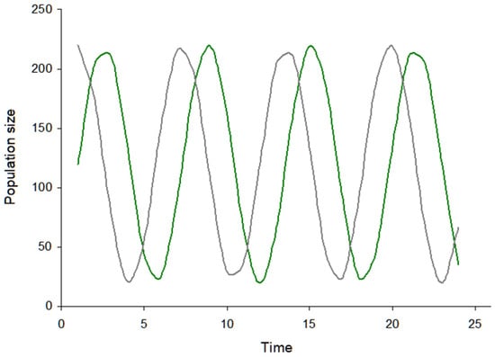
Figure 1. Plot of population dynamics in the two population system with a pathogenic virus and a vertebrate animal host. The green color line corresponds to the pathogenic virus population, while the grey color corresponds to the vertebrate host. The population dynamics originate from the Lotka–Volterra model. For example, with an increase in virus population size, the susceptible host population undergoes a decrease in size. Furthermore, the oscillations are asynchronous, reflective of the lag in time for each of the populations to respond to the other.

A central characteristic in Figure 1 is the time lag in the population response, and that the population dynamics are not synchronized with time. Where the time delay is smaller, these population oscillations are dampened. Likewise, with a larger time delay, the oscillations become larger.

Figure 2 is a plot of the population dynamics of predator and prey. Instead of displaying the populations as separate plots, as in the Figure 1, both populations are shown together in this case. The plot shows a population cycling and the long-term stability in the system. If the cycle increases in size, then the chance increases that a population may crash. If this occurs, then the system collapses and no further changes can occur in either of the populations.

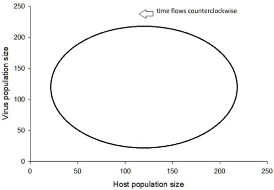
Figure 2. Cycling of pathogenic virus and vertebrate animal host populations. This result is determined by the Lotka–Volterra model of a predator-prey interaction, and the cycle persists indefinitely, given the assumptions of the model are not violated.

Instability in the predator-prey system occur by a variety of natural processes. In the case of a virus–host interaction, instability can be caused by a lack of response by evolutionary change in the pathogenic virus population, given that the vertebrate host is responding by acquiring immunity to resist the virus. This occurrence would lead to a lack of susceptible hosts (Figure 3). A different scenario is where the virus is evolving, but the vertebrate host is not adapting by acquiring immunity to the virus, and, therefore, the host population is more likely to collapse (Figure 3). In a case that is intermediate between these two scenarios, where the virus is evolving and the host is acquiring immunity, then the system may persist over time, along with the expected population oscillations.

Figure 3. Cycling in the the sizes of two populations, including the pathogenic virus and vertebrate animal host. The cycle does not persist indefinitely in this example, but instead the cycle collapses, and the host population size reaches zero. Without any susceptible hosts to infect, then the virus population will consequently collapse.

The range of possible population responses vary. In the case of a stable system with a low rate of genetic change in the virus population, and given the susceptible host population is infrequently infected, or slowly acquiring immunity, then the population oscillations will increase in size. For the common Influenza viruses, these population dynamics coincide with the seasonal changes, and, therefore, the population responses typically occur over a span of weeks or longer.

The above model shows that a virus population size can reach zero, for the case where a population crashes or is otherwise no longer participating in the system, such as where the vertebrate host population acquires immunity. However, this model also has an assumption of spatial homogeneity in the distribution of its population (Figure 4A).

Figure 4. (A). An abstract view of a population with individuals that are uniformly distributed. This illustrates an example of spatial homogeneity in a population. (B). The individuals of a population are not uniformly distributed. This is an example of spatial heterogeneity.

If instead the host population is heterogeneous in its spatial distribution, then it is expected that these populations have greater resistance to collapse (Figure 4B) ^[15]. However, this model is not applicable where there is more than one host in the system. If the virus predates on other vertebrate animal hosts, particularly if the species are taxonomically distant, then the virus is expected to maintain its population over a longer time period since the populations are spatially heterogeneous ^[15]. Likewise, an assumption of spatial homogeneity corresponds to a fairly uniform distance between individuals, but a heterogeneous pattern has a broader distribution where the expected distance is potentially greater among individuals, so, in the case of a prey population, there is a greater opportunity for hiding from predators (Figure 5). This effectively deters destabilization in this two population system.

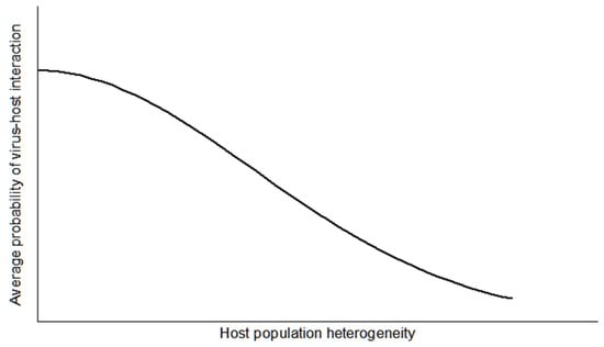
Figure 5. The plot represents a virus–host interaction, and shows that as the vertebrate host population increases in spatial or temporal heterogeneity, then the average chance of the virus–host interaction decreases. Likewise, as the heterogenity decreases, and, therefore, the host population becomes more homogeneous, then the average chance of a virus–host interaction increases. This effect illustrates the concept of predator avoidance by prey hiding from detection.

Lastly, the heterogeneity in population distribution can also occur along the temporal dimension. If the host population has individuals that are moving over time across their geographical location, then this effect is expected to lead to clustering of individuals, and potentially decrease the probability of interaction between the predator and prey.

3.3. Further Comments on Virus–Host System Instability

The above section introduces causes of instability in the virus–host population system. These causes include factors related to the evolution of new viral genotypes and the population distributions. Both of these phenomena are a result of evolutionary and ecological effects. However, these two kinds of effects are intertwined in population systems ^[6]^[7]. For instance, with a change in the natural environment, such as a change in the climatic conditions, then there exists an ecological factor that influences the virus–host system, and the factor may interact with the population responses by the virus and host. This is an additional layer of complexity for modeling the system, but is relevant for anticipating the virus–host dynamics that occur in Nature. Otherwise, oversimplication in the design of a model may lead to false expectations, particularly where the model is not robust to the missing parameters.

This is particularly relevant where associating population dynamics at the genetic level with the observed phenotypic traits. The dynamics involve factors associated with both ecology and evolution. An example of evolutionary factors is expectations on mutation and recombination rates in the populations, while ecological factors may include population distribution and interactions with the natural environment ^[6]^[7].

These systems are, at their essence, a contest of response times. Given the constraints in a virus–host system, then a delay in one of the population responses may lead to collapse of the system. If the delay is exceedingly long in comparison to the average response, then it is expected that the system will collapse. Persistence and stability of the system is increased where particular constraints are removed in the virus–host model, such as the inclusion of another host that is susceptible to the virus. Another form of escape is for the virus to more rapidly explore the space of adaptive changes and overcome any population response by the host. This may involve the mechanism of genetic recombination which complements the role of mutation in the evolutionary (and ecological) contest where the host is also responding by generation of immunity by a somatic form of recombination.

4. Model of Virus–Host Interactions at the Genetic Level

In a conventional predatory-prey interaction, the predator population responds by an increase in offspring production where the rate of growth is increasing in the prey population. Likewise, the pathogenic virus population is expected to respond by a positive growth rate with an increase in the number of susceptible vertebrate hosts. The growth in number of susceptible hosts occurs by many causes. The causes include an inadequate immune response and decay of immunity from prior virus infection.

At the mechanistic level, the vertebrate host responds by immunity at the somatic level. This response is largely based on creating a diverse number of protein receptors on dedicated immune cells. These cellular specific receptors are diverse in their protein structure as a result of mutational and recombinational processes along segments of genes in the genome of the somatic cell. However, in the case of the virus, it is expected to respond at an evolutionary level, otherwise this predator-prey system would tend toward instability, and collapse, since the availability of hosts is expected to decrease as they acquire immunity or the infection leads to host extinction. Another scenario is that the host survives with some loss of immunity and the unchanged virus type subsequently reinfects the host. This event is highly unlikely since the virus is undergoing evolution, such as by mutation, a process that is inescapable for any genetic molecule subjected to the physical processes occurring across the Earth’s biosphere.

Another factor affecting virus population response is genetic heterogeneity (Figure 6) ^[6]^[7]. If the virus population has high genetic heterogeneity (Figure 6B), then the virus is expected to have a higher chance of infecting a virus-susceptible host population. Vertebrate host populations in Nature are genetically heterogeneous, particularly in molecules that interact with pathogenic peptides, therefore, this heterogeneity is probably a necessary component as a defense against intracellular pathogens ^[6]. Likewise, a pathogenic virus population with higher genetic variation is expected to grant Nature a greater opportunity to select for variants with higher fitness.

Figure 6. (A). The circle represents a population, and the grey color boxes are the individuals with the same genotype. (B). In this case, the genotypes vary among individuals in the population. These genetic differences may be referred to as genotypic heterogeneity.

Emergence of a new viral genotype that rises relatively rapidly in the population is an example of the natural selection process of evolution. Although small populations may have a non-beneficial viral variant rise in frequency by chance, this process is expected to occur over a much longer time period (slow evolutionary rate). In the case where the natural selection process occurs repeatedly ^[16], then a large number of new or rare mutations are expected to become common in the population (high evolutionary rate).

Since the evolutionary process in small populations is not dominated by natural selection, the dynamics of gene frequencies will tend to produce non-beneficial or harmful effects in protein encoded genes (Figure 7A); the accumulation of these particular mutations will tend to lower the overall fitness of members of the population ^[17]. Recombination is an evolutionary process to escape from this dilemma and compensate for the accumulation of deleterious mutations, and, therefore, new genotypes are more easily formed with higher fitness (Figure 7B). These are probabilistic processes dependent on sampling effects in the population.

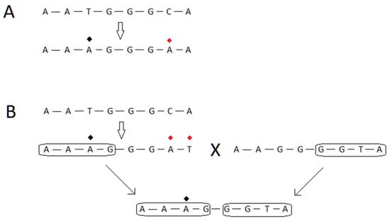
Figure 7. (A) The topmost nucleic acid sequence represents a region of a gene in a virus. The arrow points to another sequence which occurs after evolution acts on the region. The red diamond refers to a mutation that is is harmful to the fitness of the virus, while the black diamond refers to a beneficial mutation. (B) This panel is annotated the same as in (A). In this case, the topmost arrow points from a genetic sequence to one where there is one beneficial and two harmful mutations. The large letter X refers to a process of recombination, and the sequences to either side of the X are the genetic sources for the recombinational event. The genetic sequence produced from this event is shown in the bottommost portion of the panel, and the two arrows, along with the circled regions, show the source and target of the recombinational event. For one of the regions in the product, the source is shown as A-A-A-G, and the product inherits the same genetic sequence. The purpose of the panel is to show that the recombinant genetic sequence inherits the beneficial mutation from a source, but purges two harmful mutations by the recombinational process.

The shape and function of a protein is dependent on its underlying sequence of amino acids. The biological set of amino acids cluster by their chemical properties, therefore, some amino acid changes have less impact on the protein than others. In addition, for a nucleic acid sequence that codes for a protein, some of the nucleic acid changes do not result in an amino acid change (Figure 8), so it can be stated that the coding of amino acids by nucleic acids is buffered against the effects of mutation ^[18]. This is a piece of evidence for the high likelihood for the harmful effects of mutation, particularly in mutation that affects the protein sequence. Other evidence includes observation in the rates of evolution, where populations strongly disfavor amino acid change as compared to nucleic acid change that does not change the protein sequence ^[17].

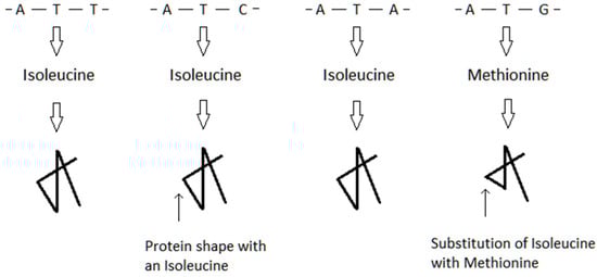
Figure 8. The genetic codons are shown across the topmost portion of the figure. These codons are translated to the amino acid isoleucine in three of the cases, and methionine in the fourth case. The purpose of the figure is to show a folded protein where one of the amino acid sites are either isoleucine or methionine. The bottommost arrows point to the location of this site in the protein shape. In this example, the replacement of isoleucine with methionine leads to a conformational change in the protein. The change of protein shape may lead to a change or loss of biological function.

References

Campillo-Balderas, J.A.; Lazcano, A.; Becerra, A. Viral genome size distribution does not correlate with the antiquity of the host lineages. Front. Ecol. Evol. 2015, 3, 143.
Sun, S.; Rao, V.B.; Rossmann, M.G. Genome packaging in viruses. Curr. Opin. Struct. Biol. 2010, 20, 114–120.
Chirico, N.; Vianelli, A.; Belshaw, R. Why genes overlap in viruses. Proc. R. Soc. B Biol. Sci. 2010, 277, 3809–3817.
Nasir, A.; Romero-Severson, E.; Claverie, J.M. Investigating the Concept and Origin of Viruses. Trends Microbiol. 2020, 28, 959–967.
Obermeyer, F.; Jankowiak, M.; Barkas, N.; Schaffner, S.F.; Pyle, J.D.; Yurkovetskiy, L.; Bosso, M.; Park, D.J.; Babadi, M.; MacInnis, B.L.; et al. Analysis of 6.4 million SARS-CoV-2 genomes identifies mutations associated with fitness. Science 2021, 376, 1327–1332.
Hamilton, W.D.; Axelrod, R.; Tanese, R. Sexual reproduction as an adaptation to resist parasites (A Review). Proc. Natl. Acad. Sci. USA 1990, 87, 3566–3573.
Agrawal, A.; Lively, C.M. Infection genetics: Gene-for-gene versus matching-alleles models and all points in between. Evol. Ecol. Res. 2002, 4, 91–107.
Anderson, R.M.; May, R.M. Coevolution of hosts and parasites. Parasitology 1982, 85, 411–426.
Lotka, A.J. Analytical note on certain rhythmic relations in organic systems. Proc. Natl. Acad. Sci. USA 1920, 6, 410–415.
Lotka, A.J. Contribution to the mathematical theory of capture: I. Conditions for capture. Proc. Natl. Acad. Sci. USA 1932, 18, 172–178.
Volterra, V. Fluctuations in the abundance of a species considered mathematically. Nature 1926, 118, 558–560.
Volterra, V. Variazioni e fluttuazioni del numero d’individui in specie animali conviventi. Mem. Della R. Accad. Naz. Dei Lincei 1926, 2, 31–113.
Kingsland, S.; Alfred, J. Lotka and the origins of theoretical population ecology. Proc. Natl. Acad. Sci. USA 2015, 112, 9493–9495.
Anisiu, M.C. Lotka, Volterra and their model. Didact. Math. 2014, 32, 9–17.
Huffaker, C. Experimental studies on predation: Dispersion factors and predator-prey oscillations. Hilgardia 1958, 27, 343–383.
Simonsen, K.L.; Churchill, G.A.; Aquadro, C.F. Properties of statistical tests of neutrality for DNA polymorphism data. Genetics 1995, 141, 413–429.
Kimura, M. The Neutral Theory of Molecular Evolution. Sci. Am. 1979, 241, 98–129.
Freeland, S.J.; Hurst, L.D. The Genetic Code Is One in a Million. J. Mol. Evol. 1998, 47, 238–248.

© Text is available under the terms and conditions of the Creative Commons Attribution (CC BY)license; additional terms may apply. By using this site, you agree to the Terms and Conditions and Privacy Policy.

Upload a video for this entry

Information

Subjects: Immunology

Contributor MDPI registered users' name will be linked to their SciProfiles pages. To register with us, please refer to https://encyclopedia.pub/register :

Robert Friedman

View Times: 200

Update Date: 14 Nov 2022

Table of Contents

Video Upload Options

Confirm