Video Upload Options

1. Separable First-order Ordinary Differential Equations

Equations in the form [math]\displaystyle{ \frac{dy}{dx} = f(x)g(y) }[/math] are called separable and are solved by [math]\displaystyle{ \frac{dy}{g(y)} = f(x)\,dx }[/math] and thus [math]\displaystyle{ \int\frac{dy}{g(y)} = \int f(x)\,dx }[/math]. Prior to dividing by [math]\displaystyle{ g(y) }[/math], one needs to check if there are stationary (also called equilibrium) solutions [math]\displaystyle{ y=\text{const} }[/math] satisfying [math]\displaystyle{ g(y)=0 }[/math].

2. Separable (Homogeneous) First-Order Linear Ordinary Differential Equations

A separable linear ordinary differential equation of the first order must be homogeneous and has the general form

[math]\displaystyle{ \frac{dy}{dt} + f(t) y = 0 }[/math]

where [math]\displaystyle{ f(t) }[/math] is some known function. We may solve this by separation of variables (moving the y terms to one side and the t terms to the other side),

[math]\displaystyle{ \frac{dy}{y} = -f(t)\, dt }[/math]

Since the separation of variables in this case involves dividing by y, we must check if the constant function y=0 is a solution of the original equation. Trivially, if y=0 then y′=0, so y=0 is actually a solution of the original equation. We note that y=0 is not allowed in the transformed equation.

We solve the transformed equation with the variables already separated by integrating,

[math]\displaystyle{ \ln |y| = \left(-\int f(t)\,dt\right) + C }[/math]

where C is an arbitrary constant. Then, by exponentiation, we obtain

[math]\displaystyle{ y = \pm e^{\left(-\int f(t)\,dt\right) + C} = \pm e^{C} e^{-\int f(t)\,dt} }[/math].

Here, [math]\displaystyle{ e^{C}\gt 0 }[/math], so [math]\displaystyle{ \pm e^{C}\neq 0 }[/math]. But we have independently checked that y=0 is also a solution of the original equation, thus

[math]\displaystyle{ y = A e^{-\int f(t)\,dt} }[/math].

with an arbitrary constant A, which covers all the cases. It is easy to confirm that this is a solution by plugging it into the original differential equation:

[math]\displaystyle{ \frac{dy}{dt} + f(t) y = -f(t) \cdot A e^{-\int f(t)\,dt} + f(t) \cdot A e^{-\int f(t)\,dt} = 0 }[/math]

Some elaboration is needed because ƒ(t) might not even be integrable. One must also assume something about the domains of the functions involved before the equation is fully defined. The solution above assumes the real case.

If [math]\displaystyle{ f(t)=\alpha }[/math] is a constant, the solution is particularly simple, [math]\displaystyle{ y = A e^{-\alpha t} }[/math] and describes, e.g., if [math]\displaystyle{ \alpha\gt 0 }[/math], the exponential decay of radioactive material at the macroscopic level. If the value of [math]\displaystyle{ \alpha }[/math] is not known a priori, it can be determined from two measurements of the solution. For example,

[math]\displaystyle{ \frac{dy}{dt} + \alpha y = 0, y(1)=2, y(2)=1 }[/math]

gives [math]\displaystyle{ \alpha = \ln(2) }[/math] and [math]\displaystyle{ y = 4 e^{-\ln(2) t}= 2^{2-t} }[/math].

3. Non-Separable (Non-Homogeneous) First-Order Linear Ordinary Differential Equations

First-order linear non-homogeneous ordinary differential equations (ODEs) are not separable. They can be solved by the following approach, known as an integrating factor method. Consider first-order linear ODEs of the general form:

[math]\displaystyle{ \frac{dy}{dx} + p(x)y = q(x) }[/math]

The method for solving this equation relies on a special integrating factor, μ:

[math]\displaystyle{ \mu = e^{\int_{x_0}^x p(t)\, dt} }[/math]

We choose this integrating factor because it has the special property that its derivative is itself times the function we are integrating, that is:

[math]\displaystyle{ \frac{d{\mu}}{dx} = e^{\int_{x_0}^x p(t)\, dt} \cdot p(x) = \mu p(x) }[/math]

Multiply both sides of the original differential equation by μ to get:

[math]\displaystyle{ \mu{\frac{dy}{dx}} + \mu{p(x)y} = \mu{q(x)} }[/math]

Because of the special μ we picked, we may substitute dμ/dx for μ p(x), simplifying the equation to:

[math]\displaystyle{ \mu{\frac{dy}{dx}} + y{\frac{d{\mu}}{dx}} = \mu{q(x)} }[/math]

Using the product rule in reverse, we get:

[math]\displaystyle{ \frac{d}{dx}{(\mu{y})} = \mu{q(x)} }[/math]

Integrating both sides:

[math]\displaystyle{ \mu{y} = \left(\int\mu q(x)\, dx\right) + C }[/math]

Finally, to solve for y we divide both sides by μ:

[math]\displaystyle{ y = \frac{\left(\int\mu q(x)\, dx\right) + C}{\mu} }[/math]

Since μ is a function of x, we cannot simplify any further directly.

4. Second-Order Linear Ordinary Differential Equations

4.1. A Simple Example

Suppose a mass is attached to a spring which exerts an attractive force on the mass proportional to the extension/compression of the spring. For now, we may ignore any other forces (gravity, friction, etc.). We shall write the extension of the spring at a time t as x(t). Now, using Newton's second law we can write (using convenient units):

[math]\displaystyle{ m\frac{d^2x}{dt^2} +kx=0, }[/math]

where m is the mass and k is the spring constant that represents a measure of spring stiffness. For simplicity's sake, let us take m=k as an example.

If we look for solutions that have the form [math]\displaystyle{ Ce^{\lambda t} }[/math], where C is a constant, we discover the relationship [math]\displaystyle{ \lambda^2+1=0 }[/math], and thus [math]\displaystyle{ \lambda }[/math] must be one of the complex numbers [math]\displaystyle{ i }[/math] or [math]\displaystyle{ -i }[/math]. Thus, using Euler's formula we can say that the solution must be of the form:

[math]\displaystyle{ x(t) = A \cos t + B \sin t }[/math]

See a solution by WolframAlpha.

To determine the unknown constants A and B, we need initial conditions, i.e. equalities that specify the state of the system at a given time (usually t = 0).

For example, if we suppose at t = 0 the extension is a unit distance (x = 1), and the particle is not moving (dx/dt = 0). We have

[math]\displaystyle{ x(0) = A \cos 0 + B \sin 0 = A = 1, }[/math]

and so A = 1.

[math]\displaystyle{ x'(0) = -A \sin 0 + B \cos 0 = B = 0, }[/math]

and so B = 0.

Therefore x(t) = cos t. This is an example of simple harmonic motion.

See a solution by Wolfram Alpha.

4.2. A More Complicated Model

The above model of an oscillating mass on a spring is plausible but not very realistic: in practice, friction will tend to decelerate the mass and have magnitude proportional to its velocity (i.e. dx/dt). Our new differential equation, expressing the balancing of the acceleration and the forces, is

[math]\displaystyle{ m\frac{d^2x}{dt^2} + c \frac{dx}{dt} + kx=0, }[/math]

where [math]\displaystyle{ c }[/math] is the damping coefficient representing friction. Again looking for solutions of the form [math]\displaystyle{ Ce^{\lambda t} }[/math], we find that

[math]\displaystyle{ m\lambda^2 + c \lambda + k = 0. }[/math]

This is a quadratic equation which we can solve. If [math]\displaystyle{ c^2\lt 4km }[/math] there are two complex conjugate roots a ± ib, and the solution (with the above boundary conditions) will look like this:

[math]\displaystyle{ x(t) = e^{at} \left(\cos bt - \frac{a}{b} \sin bt \right) }[/math]

Let us for simplicity take [math]\displaystyle{ m=1 }[/math], then [math]\displaystyle{ 0\lt c=-2a }[/math] and [math]\displaystyle{ k=a^2+b^2 }[/math].

The equation can be also solved in MATLAB symbolic toolbox as

x = dsolve('D2x+c*Dx+k*x=0','x(0)=1','Dx(0)=0') % or equivalently syms x(t) c k Dx = diff(x, t); x = dsolve(diff(x,t,2) + c*Dx + k*x == 0, x(0) == 1, Dx(0) == 0)

although the solution looks rather ugly,

x = (c + (c^2 - 4*k)^(1/2))/(2*exp(t*(c/2 - (c^2 - 4*k)^(1/2)/2))*(c^2 - 4*k)^(1/2)) - (c - (c^2 - 4*k)^(1/2))/(2*exp(t*(c/2 + (c^2 - 4*k)^(1/2)/2))*(c^2 - 4*k)^(1/2))

This is a model of a damped oscillator. The plot of displacement against time would look like this:

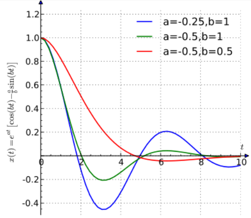
which resembles how one would expect a vibrating spring to behave as friction removes energy from the system.

5. Linear Systems of ODEs

The following example of a first order linear systems of ODEs

[math]\displaystyle{ y_1'=y_1+2y_2+t }[/math]

[math]\displaystyle{ y_2'=2y_1-2y_2+\sin(t) }[/math]

can be easily solved symbolically using numerical-analysis software.