1. Mathematical Derivation^[1][2]

From the figure the received line of sight component may be written as

[math]\displaystyle{ r_{los}(t)=Re \left\{ \frac{ \lambda \sqrt{G_{los}} }{4\pi}\times \frac{s(t) e^{-j2\pi l/\lambda}}{l} \right\} }[/math]

and the ground reflected component may be written as

[math]\displaystyle{ r_{gr}(t)=Re\left\{\frac{\lambda \Gamma(\theta) \sqrt{G_{gr}}}{4\pi}\times \frac{s(t-\tau) e^{-j2\pi (x+x')/\lambda}}{x+x'} \right\} }[/math]

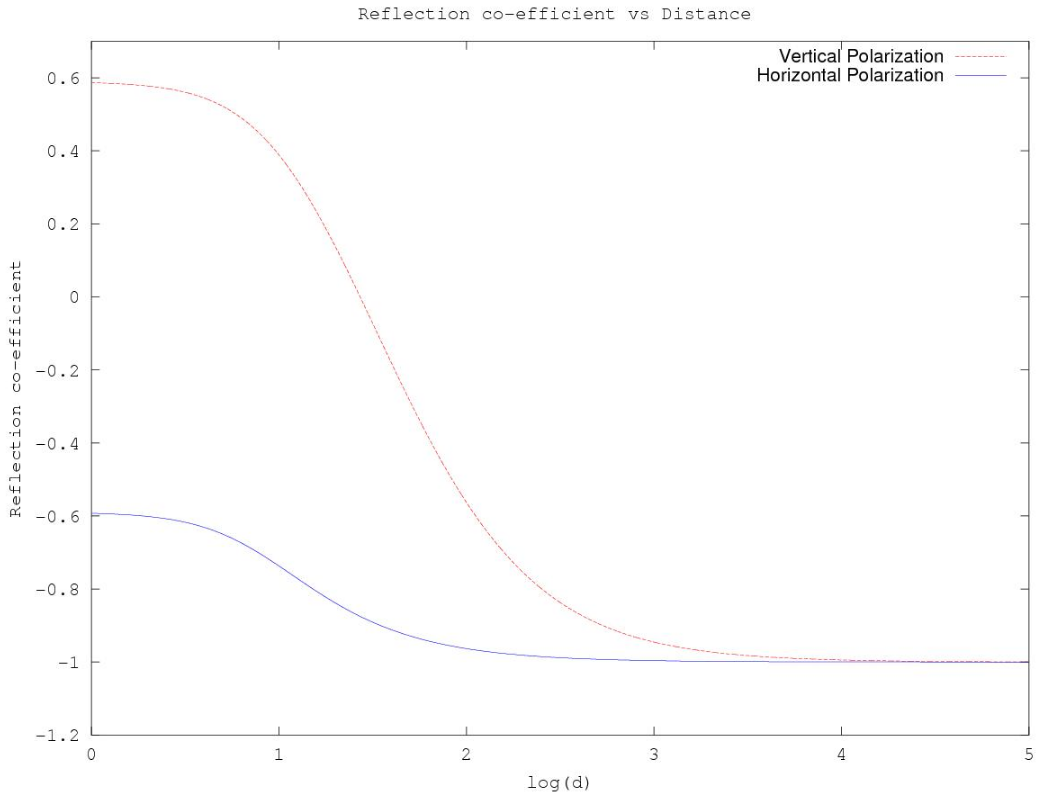
where [math]\displaystyle{ s(t) }[/math] is the transmitted signal, [math]\displaystyle{ l }[/math] is the length of the direct line-of-sight (LOS) ray, [math]\displaystyle{ x + x' }[/math] is the length of the ground-reflected ray, [math]\displaystyle{ G_{los} }[/math] is the combined antenna gain along the LOS path, [math]\displaystyle{ G_{gr} }[/math] is the combined antenna gain along the ground-reflected path, [math]\displaystyle{ \lambda }[/math] is the wavelength of the transmission ([math]\displaystyle{ \lambda = \frac{c}{f} }[/math], where [math]\displaystyle{ c }[/math] is the speed of light and [math]\displaystyle{ f }[/math] is the transmission frequency), [math]\displaystyle{ \Gamma(\theta) }[/math] is ground reflection coefficient and [math]\displaystyle{ \tau }[/math] is the delay spread of the model which equals [math]\displaystyle{ (x+x'-l)/c }[/math]. The ground reflection coefficient is^[1]

[math]\displaystyle{ \Gamma(\theta)= \frac{\sin \theta - X}{\sin \theta + X } }[/math]

where [math]\displaystyle{ X=X_h }[/math] or [math]\displaystyle{ X=X_v }[/math] depending if the signal is horizontal or vertical polarized, respectively. [math]\displaystyle{ X }[/math] is computed as follows.

[math]\displaystyle{ X_{h}=\sqrt{\varepsilon_{g}-{\cos}^2 \theta},\ X_{v}= \frac{\sqrt{\varepsilon_g-{\cos}^{2}\theta}}{\varepsilon_{g}} = \frac{X_h}{\varepsilon_g} }[/math]

The constant [math]\displaystyle{ \varepsilon_g }[/math] is the relative permittivity of the ground (or generally speaking, the material where the signal is being reflected), [math]\displaystyle{ \theta }[/math] is the angle between the ground and the reflected ray as shown in the figure above.

From the geometry of the figure, yields:

[math]\displaystyle{ x+x'=\sqrt{(h_t+h_r)^2 +d^2} }[/math]

and

[math]\displaystyle{ l=\sqrt{(h_t - h_r) ^2 +d^2} }[/math],

Therefore, the path-length difference between them is

[math]\displaystyle{ \Delta d=x+x'-l=\sqrt{(h_t+h_r )^2 +d^2}-\sqrt{(h_t- h_r) ^2 +d^2} }[/math]

and the phase difference between the waves is

[math]\displaystyle{ \Delta \phi =\frac{2 \pi \Delta d}{\lambda} }[/math]

The power of the signal received is

[math]\displaystyle{ P_r = E\{|r_{los}(t) + r_{gr}(t)|^2 \} }[/math]

where [math]\displaystyle{ E\{\cdot\} }[/math] denotes average (over time) value.

1.1. Approximation

If the signal is narrow band relative to the inverse delay spread [math]\displaystyle{ 1/\tau }[/math], so that [math]\displaystyle{ s(t)\approx s(t-\tau) }[/math], the power equation may be simplified to

[math]\displaystyle{ \begin{align} P_r= E\{|s(t)|^2\} \left( {\frac{\lambda}{4\pi}} \right) ^2 \times \left| \frac{\sqrt{G_{los}} \times e^{-j2\pi l/\lambda}}{l} + \Gamma(\theta) \sqrt{G_{gr}} \frac{e^{-j2\pi (x+x')/\lambda}}{x+x'} \right|^2&=P_t \left( {\frac{\lambda}{4\pi}} \right) ^2 \times \left| \frac{\sqrt{G_{los}}} {l} + \Gamma(\theta) \sqrt{G_{gr}} \frac{e^{-j \Delta d}}{x+x'} \right|^2 \end{align} }[/math]

where [math]\displaystyle{ P_t= E\{|s(t)|^2\} }[/math] is the transmitted power.

When distance between the antennas [math]\displaystyle{ d }[/math] is very large relative to the height of the antenna we may expand [math]\displaystyle{ \Delta d = x+x'-l }[/math],

[math]\displaystyle{ \begin{align} \Delta d = x+x'-l = d \Bigg(\sqrt{\frac{(h_t+h_r) ^2}{d^2}+1}-\sqrt{\frac{(h_t- h_r )^2 }{d^2}+1}\Bigg) \end{align} }[/math]

using the Taylor series of [math]\displaystyle{ \sqrt{1 + x} }[/math]:

[math]\displaystyle{ \sqrt{1 + x} = 1 + \textstyle \frac{1}{2}x - \frac{1}{8}x^2 + \dots, }[/math]

and taking the first two terms only,

[math]\displaystyle{ x+x'-l \approx \frac{d}{2} \times \left( \frac{(h_t+ h_r )^2}{d^2} -\frac{(h_t- h_r )^2 }{d^2} \right) = \frac{2 h_t h_r }{d} }[/math]

The phase difference can then be approximated as

[math]\displaystyle{ \Delta \phi \approx \frac{4 \pi h_t h_r }{\lambda d} }[/math]

When [math]\displaystyle{ d }[/math] is large, [math]\displaystyle{ d \gg (h_t+h_r) }[/math],

Reflection co-efficient tends to -1 for large d.

[math]\displaystyle{ \begin{align} d & \approx l \approx x+x',\ \Gamma(\theta) \approx -1,\ G_{los} \approx G_{gr} = G \end{align} }[/math]

and hence

[math]\displaystyle{ P_r \approx P_t \left( {\frac{\lambda \sqrt{G}}{4\pi d}} \right) ^2 \times | 1-e^{-j \Delta \phi}|^2 }[/math]

Expanding [math]\displaystyle{ e^{-j\Delta \phi} }[/math]using Taylor series

[math]\displaystyle{ e^x = \sum_{n=0}^\infty \frac{x^n}{n!} = 1 + x + \frac{x^2}{2} + \frac{x^3}{6} + \cdots }[/math]

and retaining only the first two terms

[math]\displaystyle{ e^{-j\Delta \phi} \approx 1 + ({-j\Delta \phi}) + \cdots = 1 - j\Delta \phi }[/math]

it follows that

[math]\displaystyle{ \begin{align} P_r & \approx P_t \left( {\frac{\lambda \sqrt{G}}{4\pi d}} \right) ^2 \times |1 - (1 -j \Delta \phi) |^2 \\ & = P_t \left( {\frac{\lambda \sqrt{G}}{4\pi d}} \right) ^2 \times \Delta \phi^2 \\ & = P_t \left({\frac{\lambda \sqrt{G}}{4\pi d}} \right) ^2 \times \left(\frac{4 \pi h_t h_r }{\lambda d} \right)^2 \\ & = P_t \frac{G h_t ^2 h_r ^2}{d^4} \end{align} }[/math]

so that

[math]\displaystyle{ P_r \approx P_t \frac{G h_t ^2 h_r ^2}{d^4} }[/math]

which is accurate in the far field region, i.e. when [math]\displaystyle{ \Delta \phi \ll 1 }[/math] (angles are measured here in radians, not degrees) or, equivalently,

[math]\displaystyle{ d \gg \frac{4 \pi h_t h_r }{\lambda} }[/math]

and where the combined antenna gain is the product of the transmit and receive antenna gains, [math]\displaystyle{ G=G_t G_r }[/math]. This formula was first obtained by B.A. Vvedenskij.^[3]

Note that the power decreases with as the inverse fourth power of the distance in the far field, which is explained by the destructive combination of the direct and reflected paths, which are roughly of the same in magnitude and are 180 degrees different in phase. [math]\displaystyle{ G_t P_t }[/math] is called "effective isotropic radiated power" (EIRP), which is the transmit power required to produce the same received power if the transmit antenna were isotropic.

2. In Logarithmic Units

In logarithmic units : [math]\displaystyle{ P_{r_\text{dBm}}=P_{t_\text{dBm}}+ 10 \log_{10}(G h_t ^2 h_r ^2) - 40 \log_{10}(d) }[/math]

Path loss : [math]\displaystyle{ PL\;=P_{t_\text{dBm}}-P_{r_\text{dBm}}\;=40 \log_{10}(d)-10 \log_{10}(G h_t ^2 h_r ^2) }[/math]

3. Power Vs. Distance Characteristics

Power vs distance plot

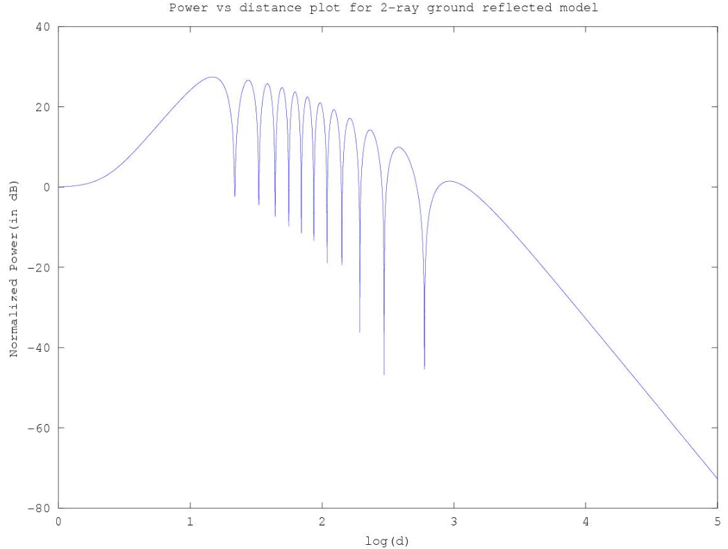
When the distance [math]\displaystyle{ d }[/math] between antennas is less than the transmitting antenna height, two waves are added constructively to yield bigger power. As distance increases, these waves add up constructively and destructively, giving regions of up-fade and down-fade. As the distance increases beyond the critical distance [math]\displaystyle{ dc }[/math] or first Fresnel zone, the power drops proportionally to an inverse of fourth power of [math]\displaystyle{ d }[/math]. An approximation to critical distance may be obtained by setting Δφ to π as the critical distance to a local maximum.

4. An Extension to Large Antenna Heights

The above approximations are valid provided that [math]\displaystyle{ d \gg (h_t+h_r) }[/math], which may be not the case in many scenarios, e.g. when antenna heights are not much smaller compared to the distance, or when the ground cannot be modelled as an ideal plane . In this case, one cannot use [math]\displaystyle{ \Gamma \approx -1 }[/math] and more refined analysis is required, see e.g.^[4]

5. As a Case of Log Distance Path Loss Model

The standard expression of Log distance path loss model is

[math]\displaystyle{ PL\;=P_{T_{dBm}}-P_{R_{dBm}}\;=\;PL_0\;+\;10\gamma\;\log_{10} \frac{d}{d_0}\;+\;X_g, }[/math]

The path loss of 2-ray ground reflected wave is

[math]\displaystyle{ PL\;=P_{t_{dBm}}-P_{r_{dBm}}\;=40 \log_{10}(d)-10 \log_{10}(G h_t ^2 h_r ^2) }[/math]

where

[math]\displaystyle{ PL_0 = 40 \log_{10}(d_0)-10 \log_{10}(G h_t ^2 h_r ^2) }[/math],

[math]\displaystyle{ X_g = 0 }[/math]

and

[math]\displaystyle{ \gamma = 4 }[/math]

for [math]\displaystyle{ d,d_0 \gt d_c }[/math] the critical distance.

6. As a Case of Multi-Slope Model

The 2-ray ground reflected model may be thought as a case of multi-slope model with break point at critical distance with slope 20 dB/decade before critical distance and slope of 40 dB/decade after the critical distance. Using the free-space and two-ray model above, the propagation path loss can be expressed as

[math]\displaystyle{ L =\max \{1,L_{FS},L_{2-ray}\} }[/math]

where [math]\displaystyle{ L_{FS}=(4\pi d/\lambda)^2 }[/math] and [math]\displaystyle{ L_{2-ray}=d^4/(h_t h_r)^2 }[/math] are the free-space and 2-ray path losses.

References

- Jakes, W.C. (1974). Microwave Mobile Communications. New York: IEEE Press.
- Rappaport, Theodore S. (2002). Wireless Communications: Principles and Practice (2. ed.). Upper Saddle River, NJ: Prentice Hall PTR. ISBN 978-0130422323.
- Vvedenskij, B.A. (December 1928). "On Radio Communications via Ultra-Short Waves". Theoretical and Experimental Electrical Engineering (12): 447–451.
- Loyka, Sergey; Kouki, Ammar (October 2001). "Using Two Ray Multipath Model for Microwave Link Budget Analysis". IEEE Antennas and Propagation Magazine 43 (5): 31–36.