1. Lemniscate Sine and Cosine Functions

1.1. Definition

The lemniscate sine (Latin: sinus lemniscatus) and lemniscate cosine (Latin: cosinus lemniscatus) functions sinlemn aka sl and coslemn aka cl are analogues of the usual sine and cosine functions, with a circle replaced by a lemniscate. They are defined by inverting integrals of algebraic functions:

[math]\displaystyle{ u=\int_0^{\operatorname{sl}(u)}\frac{dt}{\sqrt{1-t^4}} }[/math]

and

[math]\displaystyle{ u=\int_{\operatorname{cl}(u)}^1\frac{dt}{\sqrt{1-t^4}}. }[/math]

The inversion on a suitable open interval defines a real analytic function on that interval. From there, the functions are analytically extended to the complex plane. By the identity theorem, the extension is unique. The definitions can be compared to their circular counterparts:

[math]\displaystyle{ u=\int_0^{\sin (u)}\frac{dt}{\sqrt{1-t^2}} }[/math]

and

[math]\displaystyle{ u=\int_{\cos (u)}^1\frac{dt}{\sqrt{1-t^2}}. }[/math]

The lemniscatic functions are doubly periodic (or elliptic) in the complex plane, with periods 2πG and 2πiG, where Gauss's constant G is given by following expression:

[math]\displaystyle{ G= \frac{2}{\pi}\int_0^1\frac{dt}{\sqrt{1-t^4}} = 0.8346\ldots. }[/math]

In the year 1798 the German mathematician Carl Friedrich Gauss introduced the lemniscate constant:

[math]\displaystyle{ \varpi = \pi\,G = 2\int_0^1\frac{dt}{\sqrt{1-t^4}} = \int_1^\infty \frac{dt}{\sqrt{t^3-t}} = 2.622057554\ldots. }[/math]

Geometrically, the lemniscate constant is the ratio of the circumference of Bernoulli's lemniscate to its diameter (its horizontal width).

The lemniscate functions can also be defined by the Jacobi elliptic functions:

[math]\displaystyle{ \operatorname{sl}(x) = \operatorname{sn}(x;i)=\frac{1}{\sqrt{2}} \operatorname{sd}\left(\sqrt{2}x;\frac{1}{\sqrt{2}}\right) }[/math]

[math]\displaystyle{ \operatorname{cl}(x) = \operatorname{cd}(x;i)= \operatorname{cn}\left(\sqrt{2}x;\frac{1}{\sqrt{2}}\right) }[/math]

where the second arguments denote the elliptic modulus.

1.2. Arclength of Lemniscate

A lemniscate of Bernoulli and its two foci. https://handwiki.org/wiki/index.php?curid=2016096

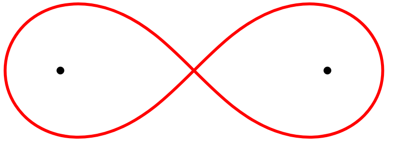
The lemniscate of Bernoulli

[math]\displaystyle{ \left(x^2+y^2\right)^2=a^2(x^2-y^2) }[/math]

consists of the points such that the product of their distances from the two points [math]\displaystyle{ (a/\sqrt{2},0) }[/math], [math]\displaystyle{ (-a/\sqrt{2},0) }[/math] is the constant [math]\displaystyle{ a^2 }[/math]. Here, [math]\displaystyle{ a }[/math] is the diameter of one lobe of the lemniscate and the points [math]\displaystyle{ (a/\sqrt{2},0) }[/math], [math]\displaystyle{ (-a/\sqrt{2},0) }[/math] are its foci. If [math]\displaystyle{ a=1 }[/math], the arc length [math]\displaystyle{ u }[/math] of the arc from the origin to a point at distance [math]\displaystyle{ s }[/math] from the origin is given by the following formula:

[math]\displaystyle{ u=\int_0^s\frac{dt}{\sqrt{1-t^4}}. }[/math]

In other words, the sine lemniscatic function gives the distance from the origin as a function of the arc length from the origin. Similarly the cosine lemniscate function gives the distance from the origin as a function of the arc length from [math]\displaystyle{ (1,0) }[/math].

Proof: In the first and the third quadrant the lemniscate of Bernoulli with [math]\displaystyle{ a=1 }[/math] can be parametrised the following way:

[math]\displaystyle{ x(s) = s\sqrt{1+s^2}/\sqrt{2} }[/math] and [math]\displaystyle{ y(s) = s\sqrt{1-s^2}/\sqrt{2} }[/math]

To calculate the arc length [math]\displaystyle{ u }[/math] the Pythagoras of the derivatives of [math]\displaystyle{ x }[/math] and [math]\displaystyle{ y }[/math] has to be formed and then integrated:

[math]\displaystyle{ u(s) = \int_0^s \sqrt{\left[\frac{d}{ds}x(s)(s = t)\right]^2 + \left[\frac{d}{ds}y(s)(s = t)\right]^2} dt = }[/math]

[math]\displaystyle{ = \int_0^s \sqrt{\left[\frac{d}{dt} t\sqrt{1+t^2}/\sqrt{2}\right]^2 + \left[\frac{d}{dt} t\sqrt{1-t^2}/\sqrt{2}\right]^2} dt = }[/math]

[math]\displaystyle{ = \int_0^s \sqrt{\frac{(1+2t^2)^2}{2(1+t^2)} + \frac{(1-2t^2)^2}{2(1-t^2)}} dt = \int_0^s \frac{1}{\sqrt{1-t^4}} dt=\operatorname{arcsl}(s) }[/math]

1.3. Properties of the Lemniscate Functions

x↦sl(x) (black) and x↦cl(x) (blue), in comparison with x↦sin⁡(πx/ϖ) (grey). https://handwiki.org/wiki/index.php?curid=1309781

[math]\displaystyle{ x\mapsto\operatorname{sl}(x) }[/math] (black) and [math]\displaystyle{ x\mapsto\operatorname{cl}(x) }[/math] (blue), in comparison with [math]\displaystyle{ x\mapsto \sin (\pi x/\varpi) }[/math] (grey)

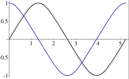
On the real line, [math]\displaystyle{ \operatorname{sl}(x)=0 }[/math] if and only if [math]\displaystyle{ x }[/math] is an integer multiple of [math]\displaystyle{ \varpi }[/math], and [math]\displaystyle{ \operatorname{cl}(x)=0 }[/math] if and only if [math]\displaystyle{ x }[/math] is an odd integer multiple of [math]\displaystyle{ \varpi /2 }[/math], so the distance between the consecutive roots of [math]\displaystyle{ x\mapsto\operatorname{sl}(x) }[/math] is [math]\displaystyle{ \varpi }[/math], and the distance between the consecutive roots of [math]\displaystyle{ x\mapsto\operatorname{cl}(x) }[/math] is [math]\displaystyle{ \varpi }[/math] as well. In other words, the role of [math]\displaystyle{ \varpi }[/math] in [math]\displaystyle{ x\mapsto\operatorname{sl}(x) }[/math] and [math]\displaystyle{ x\mapsto\operatorname{cl}(x) }[/math] is analogous to the role of [math]\displaystyle{ \pi }[/math] in [math]\displaystyle{ x\mapsto\sin (x) }[/math] and [math]\displaystyle{ x\mapsto\cos (x) }[/math].

In the complex plane, the lemniscate sine and the lemniscate cosine are meromorphic functions.

Let [math]\displaystyle{ r,s\in\mathbb{Z} }[/math]. Then for the roots we have

[math]\displaystyle{ \begin{align}\operatorname{sl}(z)&=0\iff z=r\varpi +s\varpi (i+1),\\ \operatorname{cl}(z)&=0\iff z=\frac{2r+1}{2}\varpi +s\varpi (i+1).\end{align} }[/math]

And for the poles we have

[math]\displaystyle{ \begin{align}z&\,\text{is a pole of}\,z\mapsto\operatorname{sl}(z)\iff z=r\varpi +\frac{2s+1}{2}\varpi (i+1),\\ z&\,\text{is a pole of}\,z\mapsto\operatorname{cl}(z)\iff z=\frac{2r+1}{2}\varpi +\frac{2s+1}{2}\varpi (i+1)\end{align} }[/math]

where the poles of [math]\displaystyle{ z\mapsto\operatorname{sl}(z) }[/math] are simple with residues [math]\displaystyle{ (-1)^{r+1}i }[/math] and the poles of [math]\displaystyle{ z\mapsto\operatorname{cl}(z) }[/math] are simple with residues [math]\displaystyle{ (-1)^r i }[/math].

The lemniscate sine and the lemniscate cosine have following relationship to each other:

[math]\displaystyle{ [1+\mathrm{sl}(x)^2]\cdot[1+\mathrm{cl}(x)^2] = 2 }[/math]

These are the addition theorems of the lemniscate functions:

[math]\displaystyle{ \mathrm{sl}(x+y) = \frac{\mathrm{sl}(x)\cdot\mathrm{cl}(y)+\mathrm{cl}(x)\cdot\mathrm{sl}(y)}{1-\mathrm{sl}(x)\cdot\mathrm{cl}(x)\cdot\mathrm{sl}(y)\cdot\mathrm{cl}(y)} }[/math]

[math]\displaystyle{ \arctan[\mathrm{sl}(x+y)] = \arctan[\mathrm{sl}(x)\mathrm{cl}(y)] + \arctan[\mathrm{cl}(x)\mathrm{sl}(y)] }[/math]

[math]\displaystyle{ \mathrm{cl}(x+y) = \frac{\mathrm{cl}(x)\cdot\mathrm{cl}(y)-\mathrm{sl}(x)\cdot\mathrm{sl}(y)}{1+\mathrm{sl}(x)\cdot\mathrm{cl}(x)\cdot\mathrm{sl}(y)\cdot\mathrm{cl}(y)} }[/math]

[math]\displaystyle{ \arctan[\mathrm{cl}(x+y)] = \arctan[\mathrm{cl}(x)\mathrm{cl}(y)] - \arctan[\mathrm{sl}(x)\mathrm{sl}(y)] }[/math]

The derivatives are as follows:

[math]\displaystyle{ \frac{\mathrm{d}}{\mathrm{d}x}\mathrm{sl}(x) = \mathrm{cl}(x)\cdot[1+\mathrm{sl}(x)^2] }[/math]

[math]\displaystyle{ \frac{\mathrm{d}}{\mathrm{d}x}\mathrm{cl}(x) = -\mathrm{sl}(x)\cdot[1+\mathrm{cl}(x)^2] }[/math]

The second derivatives of lemniscate sine and lemniscate cosine are their negative duplicated cubes:

[math]\displaystyle{ \frac{\mathrm{d}^2}{\mathrm{d}x^2}\mathrm{sl}(x) = -2\cdot\mathrm{sl}(x)^3 }[/math]

[math]\displaystyle{ \frac{\mathrm{d}^2}{\mathrm{d}x^2}\mathrm{cl}(x) = -2\cdot\mathrm{cl}(x)^3 }[/math]

The lemniscate functions can be integrated with the inverse tangent function:

[math]\displaystyle{ \mathrm{cl}(x)=\frac{\mathrm{d}}{\mathrm{d}x}\arctan[\mathrm{sl}(x)] }[/math]

[math]\displaystyle{ \mathrm{sl}(x)=-\frac{\mathrm{d}}{\mathrm{d}x}\arctan[\mathrm{cl}(x)] }[/math]

Halving formulas:

[math]\displaystyle{ \operatorname{sl}\left(\frac{x}{2}\right)^2 = \frac{1-\operatorname{cl}(x)\sqrt{1+\operatorname{sl}(x)^2}}{\sqrt{1+\operatorname{sl}(x)^2}+1} }[/math]

[math]\displaystyle{ \operatorname{cl}\left(\frac{x}{2}\right)^2 = \frac{1+\operatorname{cl}(x)\sqrt{1+\operatorname{sl}(x)^2}}{\sqrt{1+\operatorname{sl}(x)^2}+1} }[/math]

Duplication formulas:

[math]\displaystyle{ \operatorname{sl}(2x) = 2\,\operatorname{sl}(x)\operatorname{cl}(x)\frac{1+\operatorname{sl}(x)^2}{1+\operatorname{sl}(x)^4} }[/math]

[math]\displaystyle{ \operatorname{cl}(2x) = \frac{-1+2\,\operatorname{cl}(x)^2+\operatorname{cl}(x)^4}{1+2\,\operatorname{cl}(x)^2-\operatorname{cl}(x)^4} }[/math]

Triplication formulas:

[math]\displaystyle{ \operatorname{sl}(3x) = \frac{3\,\operatorname{sl}(x)-6\,\operatorname{sl}(x)^5-\operatorname{sl}(x)^9}{1+6\,\operatorname{sl}(x)^4-3\,\operatorname{sl}(x)^8} }[/math]

[math]\displaystyle{ \operatorname{cl}(3x) = \frac{-3\,\operatorname{cl}(x)+6\,\operatorname{cl}(x)^5+\operatorname{cl}(x)^9}{1+6\,\operatorname{cl}(x)^4-3\,\operatorname{cl}(x)^8} }[/math]

In algebraic number theory, every abelian extension of the Gaussian rationals [math]\displaystyle{ \mathbf{Q}(i) }[/math] is obtained by adjoining [math]\displaystyle{ \operatorname{sl}(\alpha) }[/math], where [math]\displaystyle{ \alpha }[/math] is a root of the equation [math]\displaystyle{ \operatorname{sl}(mu)=0 }[/math] and [math]\displaystyle{ m }[/math] is a Gaussian integer.^[1]

In terms of the Weierstrass [math]\displaystyle{ \wp }[/math]-function, the square of the lemniscate sine can be represented as

[math]\displaystyle{ \operatorname{sl}(x)^2=\frac{1}{\wp (x;4,0)}=-2\, \wp \left(\sqrt{2}x+(i-1)\frac{\Gamma ^2(1/4)}{4\sqrt{\pi}};1,0\right) }[/math]

where the second and third argument of [math]\displaystyle{ \wp }[/math] denote the lattice invariants.

1.4. Methods of Computation

The lemniscate sine can be rapidly computed by

[math]\displaystyle{ \operatorname{sl}(x)=\frac{\theta_1\left(\operatorname{M}(1,\sqrt{2})x;e^{-\pi}\right)}{\theta_3\left(\operatorname{M}(1,\sqrt{2})x;e^{-\pi}\right)} }[/math]

where

[math]\displaystyle{ \theta_1(x;q)=\sum_{n\in\mathbb{Z}}q^{(n+1/2)^2}e^{(2n+1)ix+(n-1/2)i\pi}=2\sum_{n=0}^\infty (-1)^n q^{(n+1/2)^2}\sin ((2n+1)x), }[/math]

[math]\displaystyle{ \theta_3(x;q)=\sum_{n\in\mathbb{Z}}q^{n^2}e^{2nix}=1+2\sum_{n=1}^\infty q^{n^2}\cos (2nx) }[/math]

are the Jacobi theta functions and [math]\displaystyle{ \operatorname{M} }[/math] is the arithmetic-geometric mean.

Another fast algorithm is the following:^[2] Define [math]\displaystyle{ a_0=1 }[/math] and [math]\displaystyle{ b_0=1/\sqrt{2} }[/math]. For [math]\displaystyle{ n\ge 1 }[/math], define [math]\displaystyle{ a_n=(a_{n-1}+b_{n-1})/2 }[/math], [math]\displaystyle{ b_n=\sqrt{a_{n-1}b_{n-1}} }[/math] and [math]\displaystyle{ c_n=(a_{n-1}-b_{n-1})/2 }[/math]. If [math]\displaystyle{ \phi_N=2^N a_N \sqrt{2}x }[/math] for a fixed [math]\displaystyle{ N }[/math] and

[math]\displaystyle{ \phi_{n-1}=\frac{1}{2}\phi_n+\frac{1}{2}\arcsin \left(\frac{c_n}{a_n}\sin (\phi_n)\right) }[/math]

for [math]\displaystyle{ n\ge 1 }[/math], then

[math]\displaystyle{ \operatorname{sl}(x)=\tan (\phi_0)\cos (\phi_1-\phi_0)/\sqrt{2} }[/math]

as [math]\displaystyle{ N\to\infty }[/math]. This is effectively using the arithmetic-geometric mean and is based on descending Landen's transformations.

1.5. Values of the Lemniscate Functions

This is a list of lemniscate sine and lemniscate cosine values:

[math]\displaystyle{ \mathrm{sl}\left(0\right)=0=\mathrm{cl}\left(\frac{\varpi}{2}\right) }[/math]

[math]\displaystyle{ \mathrm{sl}\left(\frac{\varpi}{2}\right)=1=\mathrm{cl}\left(0\right) }[/math]

[math]\displaystyle{ \mathrm{sl}\left(\frac{\varpi}{4}\right)=\sqrt{\sqrt{2}-1}=\mathrm{cl}\left(\frac{\varpi}{4}\right) }[/math]

[math]\displaystyle{ \mathrm{sl}\left(\frac{\varpi}{3}\right)=\sqrt[4]{2\sqrt{3}-3}=\mathrm{cl}\left(\frac{\varpi}{6}\right) }[/math]

[math]\displaystyle{ \mathrm{sl}\left(\frac{\varpi}{6}\right)=\frac{1}{2}(\sqrt{3}+1-\sqrt[4]{12})=\mathrm{cl}\left(\frac{\varpi}{3}\right) }[/math]

[math]\displaystyle{ \mathrm{sl}\left(\frac{\varpi}{8}\right)=\sqrt{(\sqrt[4]{2}-1)\left(\sqrt{2}+1-\sqrt{2+\sqrt{2}}\right)}=\mathrm{cl}\left(\frac{3\varpi}{8}\right) }[/math]

[math]\displaystyle{ \mathrm{sl}\left(\frac{3\varpi}{8}\right)=\sqrt{(\sqrt[4]{2}-1)\left(\sqrt{2}+1+\sqrt{2+\sqrt{2}}\right)}=\mathrm{cl}\left(\frac{\varpi}{8}\right) }[/math]

[math]\displaystyle{ \mathrm{sl}\left(\frac{\varpi}{5}\right)=2\sqrt[4]{\sqrt{5}-2}\sqrt{\sin\left(\frac{\pi}{20}\right)\cos\left(\frac{3\pi}{20}\right)}=\mathrm{cl}\left(\frac{3\varpi}{10}\right) }[/math]

[math]\displaystyle{ \mathrm{sl}\left(\frac{2\varpi}{5}\right)=2\sqrt[4]{\sqrt{5}-2}\sqrt{\cos\left(\frac{\pi}{20}\right)\sin\left(\frac{3\pi}{20}\right)}=\mathrm{cl}\left(\frac{\varpi}{10}\right) }[/math]

[math]\displaystyle{ \mathrm{sl}\left(\frac{\varpi}{10}\right)=\frac{1}{2}(\sqrt[4]{5}-1)\left(\sqrt{\sqrt{5}+2}-1\right)=\mathrm{cl}\left(\frac{2\varpi}{5}\right) }[/math]

[math]\displaystyle{ \mathrm{sl}\left(\frac{3\varpi}{10}\right)=\frac{1}{2}(\sqrt[4]{5}-1)\left(\sqrt{\sqrt{5}+2}+1\right)=\mathrm{cl}\left(\frac{\varpi}{5}\right) }[/math]

[math]\displaystyle{ \mathrm{sl}\left(\frac{\varpi}{12}\right)=\frac{1}{\sqrt[4]{2}}\left[\sin\left(\frac{5\pi}{24}\right)-\sqrt[4]{3}\sin\left(\frac{\pi}{24}\right)\right]\left(\sqrt[4]{2\sqrt{3}+3}-1\right)=\mathrm{cl}\left(\frac{5\varpi}{12}\right) }[/math]

[math]\displaystyle{ \mathrm{sl}\left(\frac{5\varpi}{12}\right)=\frac{1}{\sqrt[4]{2}}\left[\sin\left(\frac{5\pi}{24}\right)-\sqrt[4]{3}\sin\left(\frac{\pi}{24}\right)\right]\left(\sqrt[4]{2\sqrt{3}+3}+1\right)=\mathrm{cl}\left(\frac{\varpi}{12}\right) }[/math]

Important products for the computation of values of the modular lambda function:

[math]\displaystyle{ \mathrm{sl}\left(\frac{\varpi}{14}\right)\mathrm{sl}\left(\frac{3\varpi}{14}\right)\mathrm{sl}\left(\frac{5\varpi}{14}\right) = \frac{\sqrt[4]{\lambda^*(49)}}{\sqrt[8]{1-\lambda^*(49)^2}} = \tan\left[\frac{1}{2}\arccsc\left(\frac{1}{2}\sqrt{8\sqrt{7}+21}+\frac{1}{2}\sqrt{7}+1\right)\right] }[/math]

[math]\displaystyle{ \mathrm{sl}\left(\frac{\varpi}{18}\right)\mathrm{sl}\left(\frac{3\varpi}{18}\right)\mathrm{sl}\left(\frac{5\varpi}{18}\right)\mathrm{sl}\left(\frac{7\varpi}{18}\right) = \frac{\sqrt[4]{\lambda^*(81)}}{\sqrt[8]{1-\lambda^*(81)^2}} = \tan\left[\frac{\pi}{4}-\arctan\left(\frac{2\sqrt[3]{2\sqrt{3}-2}-2\sqrt[3]{2-\sqrt{3}}+\sqrt{3}-1}{\sqrt[4]{12}}\right)\right] }[/math]

1.6. Hyperbolic Lemniscate Functions

Definition: The hyperbolic lemniscate sine can be defined by its inverse function as follows:

[math]\displaystyle{ a = \int_{0}^{s} \frac{1}{\sqrt{t^4 + 1}} \mathrm{d}t }[/math]

[math]\displaystyle{ s = \operatorname{slh}(a) }[/math]

Analogously, the hyperbolic lemniscate cosine can be defined in this way:

[math]\displaystyle{ b = \int_{r}^{\infty} \frac{1}{\sqrt{t^4 + 1}} \mathrm{d}t }[/math]

[math]\displaystyle{ r = \operatorname{clh}(b) }[/math]

The integral from zero to infinity has following value:

[math]\displaystyle{ \int_{0}^{\infty} \frac{1}{\sqrt{t^4 + 1}} \mathrm{d}t = \frac{\varpi}{\sqrt{2}} }[/math]

Therefore, the two defined functions have following relation to each other:

[math]\displaystyle{ \operatorname{slh}(x) = \operatorname{clh}\left(\frac{\varpi}{\sqrt{2}} - x\right) }[/math]

The product of hyperbolic lemniscate sine and hyperbolic lemniscate cosine is equal to one:

[math]\displaystyle{ \mathrm{slh}(x)\,\mathrm{clh}(x) = 1 }[/math]

The hyperbolic lemniscate functions can be expressed in terms of lemniscate sine and lemniscate cosine:

[math]\displaystyle{ \mathrm{slh}(x) = \frac{\mathrm{sl}(x/\sqrt{2})\cdot[1+\mathrm{cl}(x/\sqrt{2})^2]}{\sqrt{2}\cdot\mathrm{cl}(x/\sqrt{2})} }[/math]

[math]\displaystyle{ \mathrm{clh}(x) = \frac{\mathrm{cl}(x/\sqrt{2})\cdot[1+\mathrm{sl}(x/\sqrt{2})^2]}{\sqrt{2}\cdot\mathrm{sl}(x/\sqrt{2})} }[/math]

But there is also a relation to the Jacobi elliptic functions with the elliptic modulus one by square root of two:

[math]\displaystyle{ \mathrm{slh}(x) = \frac{\operatorname{sn}(x;1/\sqrt{2})}{\operatorname{cd}(x;1/\sqrt{2})} }[/math]

[math]\displaystyle{ \mathrm{clh}(x) = \frac{\operatorname{cd}(x;1/\sqrt{2})}{\operatorname{sn}(x;1/\sqrt{2})} }[/math]

The hyperbolic lemniscate sine has following imaginary relation to the lemniscate sine:

[math]\displaystyle{ \operatorname{slh}(x) = \frac{1}{\sqrt{2}}(1-i)\operatorname{sl}\left[\frac{1}{\sqrt{2}}(1+i)x\right] }[/math]

In a superelliptic squircle of the equation [math]\displaystyle{ x^4 + y^4 = 1 }[/math] the hyperbolic lemniscate sine is defined analogously to the tangent function in a circle. If the origin point (0;0) and a point on the arc of the squircle are connected to each other by a line, the hyperbolic lemniscate sine assigns the double of the enclosed area between this line and the x-axis to the quotient of vertical coordinate of the arc point divided by its horizontal coordinate.

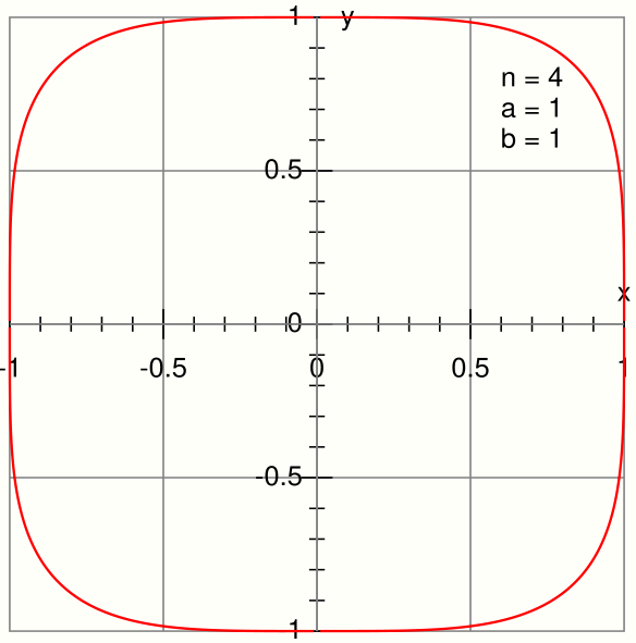Squircle of the equation x4+y4=1. https://handwiki.org/wiki/index.php?curid=2086910

Squircle of the equation [math]\displaystyle{ x^4 + y^4 = 1 }[/math]

Following addition theorem is valid for the hyperbolic lemniscate sine:

[math]\displaystyle{ \mathrm{slh}(a+b) = \frac{\mathrm{slh}(a)\sqrt{1+\mathrm{slh}(b)^4}+\mathrm{slh}(b)\sqrt{1+\mathrm{slh}(a)^4}}{1-\mathrm{slh}(a)^2\mathrm{slh}(b)^2} }[/math]

The derivative can be expressed in this way:

[math]\displaystyle{ \frac{\mathrm{d}}{\mathrm{d}x}\mathrm{slh}\,(x) = \sqrt{\mathrm{slh}\,(x)^4+1} }[/math]

2. Inverse Functions

The inverse function of the lemniscate sine is the lemniscate arcsine. This function is defined by following expression:

[math]\displaystyle{ \operatorname{arcsl}(x) = \int_{0}^{x} \frac{1}{\sqrt{1-t^4}} \mathrm{d}t }[/math]

[math]\displaystyle{ \operatorname{sl}[\operatorname{arcsl}(x)] = x }[/math]

This equation is valid for values -1 ≤ x ≤ 1.

The inverse function of the lemniscate cosine is the lemniscate arccosine. This function is defined by following expression:

[math]\displaystyle{ \operatorname{arccl}(x) = \int_{x}^{1} \frac{1}{\sqrt{1-t^4}} \mathrm{d}t }[/math]

[math]\displaystyle{ \operatorname{arccl}(x) = \frac{\varpi}{2} - \operatorname{arcsl}(x) }[/math]

[math]\displaystyle{ \operatorname{cl}[\operatorname{arccl}(x)] = x }[/math]

This equation is also valid for values -1 ≤ x ≤ 1.

The lemniscate arcsine and the lemniscate arccosine can also be expressed by the Legendre-Form:

These functions can be displayed directly by using the incomplete elliptic integral of the first kind:

[math]\displaystyle{ \operatorname{arcsl}(x) = \frac{1}{\sqrt{2}}F\left[\arcsin\left(\frac{\sqrt{2}x}{\sqrt{1+x^2}}\right);\frac{1}{\sqrt{2}}\right] }[/math]

[math]\displaystyle{ \operatorname{arcsl}(x) = 2(\sqrt{2}-1)F\left[\arcsin\left[\frac{(\sqrt{2}+1)x}{\sqrt{1+x^2}+1}\right];(\sqrt{2}-1)^2\right] }[/math]

The arc lengths of the lemniscate can also be expressed by only using the arc lengths of ellipses:

[math]\displaystyle{ \operatorname{arcsl}(x) = \frac{1}{2}(2+\sqrt{2})E\left[\arcsin\left[\frac{(\sqrt{2}+1)x}{\sqrt{1+x^2}+1}\right];(\sqrt{2}-1)^2\right] - E\left[\arcsin\left(\frac{\sqrt{2}x}{\sqrt{1+x^2}}\right);\frac{1}{\sqrt{2}}\right] + \frac{x\sqrt{1-x^2}}{\sqrt{2}(1+x^2+\sqrt{1+x^2})} }[/math]

Arc lengths of ellipses are calculated by elliptic integrals of the second kind.

The lemniscate arccosine has this expression:

[math]\displaystyle{ \operatorname{arccl}(x) = \frac{1}{\sqrt{2}}F\left[\arccos(x);\frac{1}{\sqrt{2}}\right] }[/math]

For the halving of the lemniscate arc length these formulas are valid:

[math]\displaystyle{ \operatorname{sl}\left[\frac{1}{2}\operatorname{arcsl}(x)\right] = \sin\left[\frac{1}{2}\arcsin(x)\right] \operatorname{sech}\left[\frac{1}{2}\operatorname{arsinh}(x)\right] }[/math]

[math]\displaystyle{ \operatorname{sl}\left[\frac{1}{2}\operatorname{arcsl}(x)\right]^2 = \tan\left[\frac{1}{4}\arcsin(x^2)\right] }[/math]

The lemniscate can be used to integrate many functions. Here is a list of important integrals (the constants of integration are omitted):

[math]\displaystyle{ \int\frac{1}{\sqrt{1-x^4}}\,\mathrm dx=\operatorname{arcsl}(x) }[/math]

[math]\displaystyle{ \int\frac{1}{\sqrt{(x^2+1)(2x^2+1)}}\,\mathrm dx=\operatorname{arcsl}\left(\frac{x}{\sqrt{x^2+1}}\right) }[/math]

[math]\displaystyle{ \int\frac{1}{\sqrt{x^4+6x^2+1}}\,\mathrm dx=\operatorname{arcsl}\left(\frac{\sqrt{2}x}{\sqrt{\sqrt{x^4+6x^2+1}+x^2+1}}\right) }[/math]

[math]\displaystyle{ \int\frac{1}{\sqrt{x^4+1}}\,\mathrm dx=\sqrt{2}\operatorname{arcsl}\left(\frac{x}{\sqrt{\sqrt{x^4+1}+1}}\right) }[/math]

[math]\displaystyle{ \int\frac{1}{\sqrt[4]{(1-x^4)^3}}\,\mathrm dx=\sqrt{2}\operatorname{arcsl}\left(\frac{x}{\sqrt{1+\sqrt{1-x^4}}}\right) }[/math]

[math]\displaystyle{ \int\frac{1}{\sqrt[4]{(x^4+1)^3}}\,\mathrm dx=\operatorname{arcsl}\left(\frac{x}{\sqrt[4]{x^4+1}}\right) }[/math]

[math]\displaystyle{ \int\frac{1}{\sqrt[4]{(1-x^2)^3}}\,\mathrm dx=2\operatorname{arcsl}\left(\frac{x}{1+\sqrt{1-x^2}}\right) }[/math]

[math]\displaystyle{ \int\frac{1}{\sqrt[4]{(x^2+1)^3}}\,\mathrm dx=2\operatorname{arcsl}\left(\frac{x}{\sqrt{x^2+1}+1}\right) }[/math]

[math]\displaystyle{ \int\frac{1}{\sqrt[4]{(ax^2+bx+c)^3}}\,\mathrm dx=\frac{2\sqrt{2}}{\sqrt[4]{4a^2c-ab^2}}\operatorname{arcsl}\left[\frac{2ax+b}{\sqrt{4a(ax^2+bx+c)}+\sqrt{4ac-b^2}}\right] }[/math]

[math]\displaystyle{ \int\sqrt{\operatorname{sech}(x)}\,\mathrm dx=2\operatorname{arcsl}[\tanh(x/2)] }[/math]

[math]\displaystyle{ \int\sqrt{\sec(x)}\,\mathrm dx=2\operatorname{arcsl}[\tan(x/2)] }[/math]

References

- Ogawa, Takuma (2005). "SIMILARITIES BETWEEN THE TRIGONOMETRIC FUNCTION AND THE LEMNISCATE FUNCTION FROM ARITHEMETIC VIEW POINT". https://www.jstor.org/stable/43686710?seq=1.
- Carlson, B. C. (2010), "Jacobian Elliptic Functions", in Olver, Frank W. J.; Lozier, Daniel M.; Boisvert, Ronald F. et al., NIST Handbook of Mathematical Functions, Cambridge University Press, ISBN 978-0-521-19225-5, http://dlmf.nist.gov/22.20.E5