 +1 credit
| Version | Summary | Created by | Modification | Content Size | Created at | Operation |
|---|---|---|---|---|---|---|
| 1 | Vivi Li | -- | 3439 | 2022-10-10 01:34:57 |
Video Upload Options
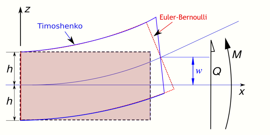
The Timoshenko-Ehrenfest beam theory was developed by Stephen Timoshenko and Paul Ehrenfest early in the 20th century. The model takes into account shear deformation and rotational bending effects, making it suitable for describing the behaviour of thick beams, sandwich composite beams, or beams subject to high-frequency excitation when the wavelength approaches the thickness of the beam. The resulting equation is of 4th order but, unlike Euler–Bernoulli beam theory, there is also a second-order partial derivative present. Physically, taking into account the added mechanisms of deformation effectively lowers the stiffness of the beam, while the result is a larger deflection under a static load and lower predicted eigenfrequencies for a given set of boundary conditions. The latter effect is more noticeable for higher frequencies as the wavelength becomes shorter (in principle comparable to the height of the beam or shorter), and thus the distance between opposing shear forces decreases. Rotary inertia effect was introduced by Bresse and Rayleigh. If the shear modulus of the beam material approaches infinity—and thus the beam becomes rigid in shear—and if rotational inertia effects are neglected, Timoshenko beam theory converges towards ordinary beam theory.
1. Quasistatic Timoshenko Beam
In static Timoshenko beam theory without axial effects, the displacements of the beam are assumed to be given by
- [math]\displaystyle{ u_x(x,y,z) = -z~\varphi(x) ~;~~ u_y(x,y,z) = 0 ~;~~ u_z(x,y) = w(x) }[/math]
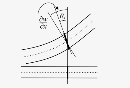
where [math]\displaystyle{ (x,y,z) }[/math] are the coordinates of a point in the beam, [math]\displaystyle{ u_x, u_y, u_z }[/math] are the components of the displacement vector in the three coordinate directions, [math]\displaystyle{ \varphi }[/math] is the angle of rotation of the normal to the mid-surface of the beam, and [math]\displaystyle{ w }[/math] is the displacement of the mid-surface in the [math]\displaystyle{ z }[/math]-direction.
The governing equations are the following coupled system of ordinary differential equations:
- [math]\displaystyle{ \begin{align} & \frac{\mathrm{d}^2}{\mathrm{d} x^2}\left(EI\frac{\mathrm{d} \varphi}{\mathrm{d} x}\right) = q(x) \\ & \frac{\mathrm{d} w}{\mathrm{d} x} = \varphi - \frac{1}{\kappa AG} \frac{\mathrm{d}}{\mathrm{d} x}\left(EI\frac{\mathrm{d} \varphi}{\mathrm{d} x}\right). \end{align} }[/math]
The Timoshenko beam theory for the static case is equivalent to the Euler-Bernoulli theory when the last term above is neglected, an approximation that is valid when
- [math]\displaystyle{ \frac{EI}{\kappa L^2 A G} \ll 1 }[/math]
where
- [math]\displaystyle{ L }[/math] is the length of the beam.
- [math]\displaystyle{ A }[/math] is the cross section area.
- [math]\displaystyle{ E }[/math] is the elastic modulus.
- [math]\displaystyle{ G }[/math] is the shear modulus.
- [math]\displaystyle{ I }[/math] is the second moment of area.
- [math]\displaystyle{ \kappa }[/math], called the Timoshenko shear coefficient, depends on the geometry. Normally, [math]\displaystyle{ \kappa = 5/6 }[/math] for a rectangular section.
- [math]\displaystyle{ q(x) }[/math] is a distributed load (force per length).
Combining the two equations gives, for a homogeneous beam of constant cross-section,
- [math]\displaystyle{ EI~\cfrac{\mathrm{d}^4 w}{\mathrm{d} x^4} = q(x) - \cfrac{EI}{\kappa A G}~\cfrac{\mathrm{d}^2 q}{\mathrm{d} x^2} }[/math]
The bending moment [math]\displaystyle{ M_{xx} }[/math] and the shear force [math]\displaystyle{ Q_x }[/math] in the beam are related to the displacement [math]\displaystyle{ w }[/math] and the rotation [math]\displaystyle{ \varphi }[/math]. These relations, for a linear elastic Timoshenko beam, are:
- [math]\displaystyle{ M_{xx} = -EI~\frac{\partial \varphi}{\partial x} \quad \text{and} \quad Q_{x} = \kappa~AG~\left(-\varphi + \frac{\partial w}{\partial x}\right) \,. }[/math]
-
Derivation of quasistatic Timoshenko beam equations From the kinematic assumptions for a Timoshenko beam, the displacements of the beam are given by - [math]\displaystyle{ u_x(x,y,z,t) = -z~\varphi(x,t) ~;~~ u_y(x,y,z,t) = 0 ~;~~ u_z(x,y,z) = w(x,t) }[/math]
Then, from the strain-displacement relations for small strains, the non-zero strains based on the Timoshenko assumptions are
- [math]\displaystyle{ \varepsilon_{xx} = \frac{\partial u_x}{\partial x} = -z~\frac{\partial \varphi}{\partial x} ~;~~ \varepsilon_{xz} = \frac{1}{2}\left(\frac{\partial u_x}{\partial z}+\frac{\partial u_z}{\partial x}\right) = \frac{1}{2}\left(-\varphi + \frac{\partial w}{\partial x}\right) }[/math]
Since the actual shear strain in the beam is not constant over the cross section we introduce a correction factor [math]\displaystyle{ \kappa }[/math] such that
- [math]\displaystyle{ \varepsilon_{xz} = \frac{1}{2}~\kappa~\left(-\varphi + \frac{\partial w}{\partial x}\right) }[/math]
The variation in the internal energy of the beam is
- [math]\displaystyle{ \delta U = \int_L \int_A (\sigma_{xx}\delta\varepsilon_{xx} + 2\sigma_{xz}\delta\varepsilon_{xz})~\mathrm{d}A~\mathrm{d}L = \int_L \int_A \left[-z~\sigma_{xx}\frac{\partial (\delta\varphi)}{\partial x} + \sigma_{xz}~\kappa\left(-\delta\varphi + \frac{\partial (\delta w)}{\partial x}\right)\right]~\mathrm{d}A~\mathrm{d}L }[/math]
Define
- [math]\displaystyle{ M_{xx} := \int_A z~\sigma_{xx}~\mathrm{d}A ~;~~ Q_x := \kappa~\int_A \sigma_{xz}~\mathrm{d}A }[/math]
Then
- [math]\displaystyle{ \delta U = \int_L \left[-M_{xx}\frac{\partial (\delta\varphi)}{\partial x} + Q_{x}\left(-\delta\varphi + \frac{\partial (\delta w)}{\partial x}\right)\right]~\mathrm{d}L }[/math]
Integration by parts, and noting that because of the boundary conditions the variations are zero at the ends of the beam, leads to
- [math]\displaystyle{ \delta U = \int_L \left[\left(\frac{\partial M_{xx}}{\partial x} - Q_x\right)~\delta\varphi - \frac{\partial Q_{x}}{\partial x}~\delta w\right]~\mathrm{d}L }[/math]
The variation in the external work done on the beam by a transverse load [math]\displaystyle{ q(x,t) }[/math] per unit length is
- [math]\displaystyle{ \delta W = \int_L q~\delta w~\mathrm{d}L }[/math]
Then, for a quasistatic beam, the principle of virtual work gives
- [math]\displaystyle{ \delta U = \delta W \implies \int_L \left[\left(\frac{\partial M_{xx}}{\partial x} - Q_x\right)~\delta\varphi - \left(\frac{\partial Q_{x}}{\partial x} + q\right)~\delta w\right]~\mathrm{d}L = 0 }[/math]
The governing equations for the beam are, from the fundamental theorem of variational calculus,
- [math]\displaystyle{ \frac{\partial M_{xx}}{\partial x} - Q_x = 0 ~;~~ \frac{\partial Q_{x}}{\partial x} + q = 0 }[/math]
For a linear elastic beam
- [math]\displaystyle{ \begin{align} M_{xx} & = \int_A z~\sigma_{xx}~\mathrm{d}A = \int_A z~E~\varepsilon_{xx}~\mathrm{d}A = -\int_A z^2~E~\frac{\partial \varphi}{\partial x}~\mathrm{d}A = -EI~\frac{\partial \varphi}{\partial x} \\ Q_{x} & = \int_A \sigma_{xz}~\mathrm{d}A = \int_A 2G~\varepsilon_{xz}~\mathrm{d}A = \int_A \kappa~G~\left(-\varphi + \frac{\partial w}{\partial x}\right)~\mathrm{d}A = \kappa~AG~\left(-\varphi + \frac{\partial w}{\partial x}\right) \end{align} }[/math]
Therefore the governing equations for the beam may be expressed as
- [math]\displaystyle{ \begin{align} \frac{\partial }{\partial x}\left(EI\frac{\partial \varphi}{\partial x}\right) + \kappa AG~\left(\frac{\partial w}{\partial x}-\varphi\right) & = 0 \\ \frac{\partial }{\partial x}\left[\kappa AG\left(\frac{\partial w}{\partial x} - \varphi\right)\right] + q & = 0 \end{align} }[/math]
Combining the two equations together gives
- [math]\displaystyle{ \begin{align} & \frac{\partial^2 }{\partial x^2}\left(EI\frac{\partial \varphi}{\partial x}\right) = q \\ & \frac{\partial w}{\partial x} = \varphi - \cfrac{1}{\kappa AG}~\frac{\partial }{\partial x}\left(EI\frac{\partial \varphi}{\partial x}\right) \end{align} }[/math]
1.1. Boundary Conditions
The two equations that describe the deformation of a Timoshenko beam have to be augmented with boundary conditions if they are to be solved. Four boundary conditions are needed for the problem to be well-posed. Typical boundary conditions are:
- Simply supported beams: The displacement [math]\displaystyle{ w }[/math] is zero at the locations of the two supports. The bending moment [math]\displaystyle{ M_{xx} }[/math] applied to the beam also has to be specified. The rotation [math]\displaystyle{ \varphi }[/math] and the transverse shear force [math]\displaystyle{ Q_x }[/math] are not specified.
- Clamped beams: The displacement [math]\displaystyle{ w }[/math] and the rotation [math]\displaystyle{ \varphi }[/math] are specified to be zero at the clamped end. If one end is free, shear force [math]\displaystyle{ Q_x }[/math] and bending moment [math]\displaystyle{ M_{xx} }[/math] have to be specified at that end.
1.2. Example: Cantilever Beam
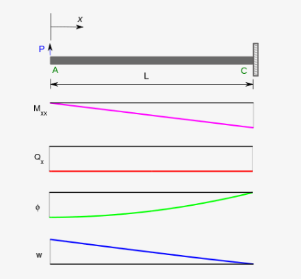
For a cantilever beam, one boundary is clamped while the other is free. Let us use a right handed coordinate system where the [math]\displaystyle{ x }[/math] direction is positive towards right and the [math]\displaystyle{ z }[/math] direction is positive upward. Following normal convention, we assume that positive forces act in the positive directions of the [math]\displaystyle{ x }[/math] and [math]\displaystyle{ z }[/math] axes and positive moments act in the clockwise direction. We also assume that the sign convention of the stress resultants ([math]\displaystyle{ M_{xx} }[/math] and [math]\displaystyle{ Q_x }[/math]) is such that positive bending moments compress the material at the bottom of the beam (lower [math]\displaystyle{ z }[/math] coordinates) and positive shear forces rotate the beam in a counterclockwise direction.
Let us assume that the clamped end is at [math]\displaystyle{ x=L }[/math] and the free end is at [math]\displaystyle{ x=0 }[/math]. If a point load [math]\displaystyle{ P }[/math] is applied to the free end in the positive [math]\displaystyle{ z }[/math] direction, a free body diagram of the beam gives us
- [math]\displaystyle{ -Px - M_{xx} = 0 \implies M_{xx} = -Px }[/math]
and
- [math]\displaystyle{ P + Q_x = 0 \implies Q_x = -P\,. }[/math]
Therefore, from the expressions for the bending moment and shear force, we have
- [math]\displaystyle{ Px = EI\,\frac{d\varphi}{dx} \qquad \text{and} \qquad -P = \kappa AG\left(-\varphi + \frac{dw}{dx}\right) \,. }[/math]
Integration of the first equation, and application of the boundary condition [math]\displaystyle{ \varphi = 0 }[/math] at [math]\displaystyle{ x = L }[/math], leads to
- [math]\displaystyle{ \varphi(x) = -\frac{P}{2EI}\,(L^2-x^2) \,. }[/math]
The second equation can then be written as
- [math]\displaystyle{ \frac{dw}{dx} = -\frac{P}{\kappa AG} - \frac{P}{2EI}\,(L^2-x^2)\,. }[/math]
Integration and application of the boundary condition [math]\displaystyle{ w = 0 }[/math] at [math]\displaystyle{ x = L }[/math] gives
- [math]\displaystyle{ w(x) = \frac{P(L-x)}{\kappa AG} - \frac{Px}{2EI}\,\left(L^2-\frac{x^2}{3}\right) + \frac{PL^3}{3EI} \,. }[/math]
The axial stress is given by
- [math]\displaystyle{ \sigma_{xx}(x,z) = E\,\varepsilon_{xx} = -E\,z\,\frac{d\varphi}{dx} = -\frac{Pxz}{I} = \frac{M_{xx}z}{I} \,. }[/math]
2. Dynamic Timoshenko Beam
In Timoshenko beam theory without axial effects, the displacements of the beam are assumed to be given by
- [math]\displaystyle{ u_x(x,y,z,t) = -z~\varphi(x,t) ~;~~ u_y(x,y,z,t) = 0 ~;~~ u_z(x,y,z,t) = w(x,t) }[/math]
where [math]\displaystyle{ (x,y,z) }[/math] are the coordinates of a point in the beam, [math]\displaystyle{ u_x, u_y, u_z }[/math] are the components of the displacement vector in the three coordinate directions, [math]\displaystyle{ \varphi }[/math] is the angle of rotation of the normal to the mid-surface of the beam, and [math]\displaystyle{ w }[/math] is the displacement of the mid-surface in the [math]\displaystyle{ z }[/math]-direction.
Starting from the above assumption, the Timoshenko beam theory, allowing for vibrations, may be described with the coupled linear partial differential equations:[1]
- [math]\displaystyle{ \rho A\frac{\partial^{2}w}{\partial t^{2}} - q(x,t) = \frac{\partial}{\partial x}\left[ \kappa AG \left(\frac{\partial w}{\partial x}-\varphi\right)\right] }[/math]
- [math]\displaystyle{ \rho I\frac{\partial^{2}\varphi}{\partial t^{2}} = \frac{\partial}{\partial x}\left(EI\frac{\partial \varphi}{\partial x}\right)+\kappa AG\left(\frac{\partial w}{\partial x}-\varphi\right) }[/math]
where the dependent variables are [math]\displaystyle{ w(x,t) }[/math], the translational displacement of the beam, and [math]\displaystyle{ \varphi(x,t) }[/math], the angular displacement. Note that unlike the Euler-Bernoulli theory, the angular deflection is another variable and not approximated by the slope of the deflection. Also,
- [math]\displaystyle{ \rho }[/math] is the density of the beam material (but not the linear density).
- [math]\displaystyle{ A }[/math] is the cross section area.
- [math]\displaystyle{ E }[/math] is the elastic modulus.
- [math]\displaystyle{ G }[/math] is the shear modulus.
- [math]\displaystyle{ I }[/math] is the second moment of area.
- [math]\displaystyle{ \kappa }[/math], called the Timoshenko shear coefficient, depends on the geometry. Normally, [math]\displaystyle{ \kappa = 5/6 }[/math] for a rectangular section.
- [math]\displaystyle{ q(x,t) }[/math] is a distributed load (force per length).
- [math]\displaystyle{ m := \rho A }[/math]
- [math]\displaystyle{ J := \rho I }[/math]
These parameters are not necessarily constants.
For a linear elastic, isotropic, homogeneous beam of constant cross-section these two equations can be combined to give[2][3]
- [math]\displaystyle{ EI~\cfrac{\partial^4 w}{\partial x^4} + m~\cfrac{\partial^2 w}{\partial t^2} - \left(J + \cfrac{E I m}{\kappa A G}\right)\cfrac{\partial^4 w}{\partial x^2~\partial t^2} + \cfrac{m J}{\kappa A G}~\cfrac{\partial^4 w}{\partial t^4} = q(x,t) + \cfrac{J}{\kappa A G}~\cfrac{\partial^2 q}{\partial t^2} - \cfrac{EI}{\kappa A G}~\cfrac{\partial^2 q}{\partial x^2} }[/math]
-
Derivation of combined Timoshenko beam equation The equations governing the bending of a homogeneous Timoshenko beam of constant cross-section are - [math]\displaystyle{ \begin{align} (1) & & \quad m~\frac{\partial^2 w}{\partial t^2} & = \kappa AG~\left(\frac{\partial^2 w}{\partial x^2} - \frac{\partial \varphi}{\partial x}\right) + q(x,t) ~;~~ m := \rho A \\ (2) & & \quad J~\frac{\partial^2 \varphi}{\partial t^2} & = EI~\frac{\partial^2 \varphi}{\partial x^2} + \kappa AG~\left(\frac{\partial w}{\partial x} - \varphi\right) ~;~~ J := \rho I \end{align} }[/math]
From equation (1), assuming appropriate smoothness, we have
- [math]\displaystyle{ \begin{align} (3) & & \quad \frac{\partial \varphi}{\partial x} & = \cfrac{q}{\kappa AG} -\cfrac{m}{\kappa AG}~\frac{\partial^2 w}{\partial t^2} + \frac{\partial^2 w}{\partial x^2} \\ (4) & & \quad \cfrac{\partial^3\varphi}{\partial x^3} &= \frac{1}{\kappa AG} \frac{\partial^2 q}{\partial x^2} - \frac{m}{\kappa AG}~\cfrac{\partial^4 w}{\partial x^2\partial t^2} + \cfrac{\partial^4 w}{\partial x^4}\\ (5) & & \quad \cfrac{\partial^3\varphi}{\partial x\partial t^2} &= \frac{1}{\kappa AG} \frac{\partial^2 q}{\partial t^2} - \frac{m}{\kappa AG}~\cfrac{\partial^4 w}{\partial t^4} + \cfrac{\partial^4 w}{\partial x^2\partial t^2} \end{align} }[/math]
Differentiating equation (2) gives
- [math]\displaystyle{ \begin{align} (6) & & \quad J~\frac{\partial^3 \varphi}{\partial x\partial t^2} & = EI~\frac{\partial^3 \varphi}{\partial x^3} + \kappa AG~\left(\frac{\partial w^2}{\partial x^2} - \frac{\partial\varphi}{\partial x} \right) \end{align} }[/math]
Substituting equation (3), (4), (5) into equation (6) and rearrange, we get
- [math]\displaystyle{ \begin{align} EI~\cfrac{\partial^4 w}{\partial x^4} + m~\frac{\partial^2 w}{\partial t^2} - \left(J+\cfrac{mEI}{\kappa AG}\right)~\cfrac{\partial^4 w}{\partial x^2 \partial t^2} + \cfrac{mJ}{\kappa AG}~\cfrac{\partial^4 w}{\partial t^4} = q + \cfrac{J}{\kappa AG}~\frac{\partial^2 q}{\partial t^2} - \cfrac{EI}{\kappa A G}~\frac{\partial^2 q}{\partial x^2} \end{align} }[/math]
The Timoshenko equation predicts a critical frequency [math]\displaystyle{ \omega_C=2 \pi f_c=\sqrt{\frac{\kappa GA}{\rho I}}. }[/math] For normal modes the Timoshenko equation can be solved. Being a fourth order equation, there are four independent solutions, two oscillatory and two evanescent for frequencies below [math]\displaystyle{ f_c }[/math]. For frequencies larger than [math]\displaystyle{ f_c }[/math] all solutions are oscillatory and, as consequence, a second spectrum appears.[4]
2.1. Axial Effects
If the displacements of the beam are given by
- [math]\displaystyle{ u_x(x,y,z,t) = u_0(x,t)-z~\varphi(x,t) ~;~~ u_y(x,y,z,t) = 0 ~;~~ u_z(x,y,z,t) = w(x,t) }[/math]
where [math]\displaystyle{ u_0 }[/math] is an additional displacement in the [math]\displaystyle{ x }[/math]-direction, then the governing equations of a Timoshenko beam take the form
- [math]\displaystyle{ \begin{align} m \frac{\partial^{2}w}{\partial t^{2}} & = \frac{\partial}{\partial x}\left[ \kappa AG \left(\frac{\partial w}{\partial x}-\varphi\right)\right] + q(x,t) \\ J \frac{\partial^{2}\varphi}{\partial t^{2}} & = N(x,t)~\frac{\partial w}{\partial x} + \frac{\partial}{\partial x}\left(EI\frac{\partial \varphi}{\partial x}\right)+\kappa AG\left(\frac{\partial w}{\partial x}-\varphi\right) \end{align} }[/math]
where [math]\displaystyle{ J = \rho I }[/math] and [math]\displaystyle{ N(x,t) }[/math] is an externally applied axial force. Any external axial force is balanced by the stress resultant
- [math]\displaystyle{ N_{xx}(x,t) = \int_{-h}^{h} \sigma_{xx}~dz }[/math]
where [math]\displaystyle{ \sigma_{xx} }[/math] is the axial stress and the thickness of the beam has been assumed to be [math]\displaystyle{ 2h }[/math].
The combined beam equation with axial force effects included is
- [math]\displaystyle{ EI~\cfrac{\partial^4 w}{\partial x^4} + N~\cfrac{\partial^2 w}{\partial x^2} + m~\frac{\partial^2 w}{\partial t^2} - \left(J+\cfrac{mEI}{\kappa AG}\right)~\cfrac{\partial^4 w}{\partial x^2 \partial t^2} + \cfrac{mJ}{\kappa AG}~\cfrac{\partial^4 w}{\partial t^4} = q + \cfrac{J}{\kappa AG}~\frac{\partial^2 q}{\partial t^2} - \cfrac{EI}{\kappa A G}~\frac{\partial^2 q}{\partial x^2} }[/math]
2.2. Damping
If, in addition to axial forces, we assume a damping force that is proportional to the velocity with the form
- [math]\displaystyle{ \eta(x)~\cfrac{\partial w}{\partial t} }[/math]
the coupled governing equations for a Timoshenko beam take the form
- [math]\displaystyle{ m \frac{\partial^{2}w}{\partial t^{2}} + \eta(x)~\cfrac{\partial w}{\partial t} = \frac{\partial}{\partial x}\left[ \kappa AG \left(\frac{\partial w}{\partial x}-\varphi\right)\right] + q(x,t) }[/math]
- [math]\displaystyle{ J \frac{\partial^{2}\varphi}{\partial t^{2}} = N\frac{\partial w}{\partial x} + \frac{\partial}{\partial x}\left(EI\frac{\partial \varphi}{\partial x}\right)+\kappa AG\left(\frac{\partial w}{\partial x}-\varphi\right) }[/math]
and the combined equation becomes
- [math]\displaystyle{ \begin{align} EI~\cfrac{\partial^4 w}{\partial x^4} & + N~\cfrac{\partial^2 w}{\partial x^2} + m~\frac{\partial^2 w}{\partial t^2} - \left(J+\cfrac{mEI}{\kappa AG}\right)~\cfrac{\partial^4 w}{\partial x^2 \partial t^2} + \cfrac{mJ}{\kappa AG}~\cfrac{\partial^4 w}{\partial t^4} + \cfrac{J \eta(x)}{\kappa AG}~\cfrac{\partial^3 w}{\partial t^3} \\ & -\cfrac{EI}{\kappa AG}~\cfrac{\partial^2}{\partial x^2}\left(\eta(x)\cfrac{\partial w}{\partial t}\right) + \eta(x)\cfrac{\partial w}{\partial t} = q + \cfrac{J}{\kappa AG}~\frac{\partial^2 q}{\partial t^2} - \cfrac{EI}{\kappa A G}~\frac{\partial^2 q}{\partial x^2} \end{align} }[/math]
A caveat to this Ansatz damping force (resembling viscosity) is that, whereas viscosity leads to a frequency-dependent and amplitude-independent damping rate of beam oscillations, the empirically measured damping rates are frequency-insensitive, but depend on the amplitude of beam deflection.
3. Shear Coefficient
Determining the shear coefficient is not straightforward (nor are the determined values widely accepted, i.e. there's more than one answer); generally it must satisfy:
- [math]\displaystyle{ \int_A \tau dA = \kappa A G \varphi\, }[/math] .
The shear coefficient depends on Poisson's ratio. The attempts to provide precise expressions were made by many scientists, including Stephen Timoshenko,[5] Raymond D. Mindlin,[6] G. R. Cowper,[7] N. G. Stephen,[8] J. R. Hutchinson[9] etc. (see also the derivation of the Timoshenko beam theory as a refined beam theory based on the variational-asymptotic method in the book by Khanh C. Le[10] leading to different shear coefficients in the static and dynamic cases). In engineering practice, the expressions by Stephen Timoshenko[11] are sufficient in most cases. In 1975 Kaneko[12] published an excellent review of studies of the shear coefficient. More recently new experimental data show that the shear coefficient is underestimated [13][14].
According to Cowper (1966) for solid rectangular cross-sections,
- [math]\displaystyle{ \kappa = \cfrac{10(1+\nu)}{12+11\nu} }[/math]
and for solid circular cross-sections,
- [math]\displaystyle{ \kappa = \cfrac{6(1+\nu)}{7+6\nu} }[/math]
where [math]\displaystyle{ \nu }[/math] is Poisson's ratio.
References
- Timoshenko's Beam Equations http://ccrma.stanford.edu/~bilbao/master/node163.html
- Thomson, W. T., 1981, Theory of Vibration with Applications, second edition. Prentice-Hall, New Jersey.
- Rosinger, H. E. and Ritchie, I. G., 1977, On Timoshenko's correction for shear in vibrating isotropic beams, J. Phys. D: Appl. Phys., vol. 10, pp. 1461-1466.
- "Experimental study of the Timoshenko beam theory predictions", A. Díaz-de-Anda, J. Flores, L. Gutiérrez, R.A. Méndez-Sánchez, G. Monsivais, and A. Morales, Journal of Sound and Vibration, Volume 331, Issue 26, 17 December 2012, pp. 5732–5744.
- Timoshenko, Stephen P., 1932, Schwingungsprobleme der Technik, Julius Springer.
- Mindlin, R. D., Deresiewicz, H., 1953, Timoshenko's Shear Coefficient for Flexural Vibrations of Beams, Technical Report No. 10, ONR Project NR064-388, Department of Civil Engineering, Columbia University, New York, N.Y.
- Cowper, G. R., 1966, "The Shear Coefficient in Timoshenko’s Beam Theory", J. Appl. Mech., Vol. 33, No.2, pp. 335–340.
- Stephen, N. G., 1980. "Timoshenko’s shear coefficient from a beam subjected to gravity loading", Journal of Applied Mechanics, Vol. 47, No. 1, pp. 121–127.
- Hutchinson, J. R., 1981, "Transverse vibration of beams, exact versus approximate solutions", Journal of Applied Mechanics, Vol. 48, No. 12, pp. 923–928.
- Le, Khanh C., 1999, Vibrations of shells and rods, Springer.
- Stephen Timoshenko, James M. Gere. Mechanics of Materials. Van Nostrand Reinhold Co., 1972. pages 207.
- Kaneko, T., 1975, "On Timoshenko's correction for shear in vibrating beams", J. Phys. D: Appl. Phys., Vol. 8, pp. 1927–1936.
- "Experimental check on the accuracy of Timoshenko’s beam theory", R. A. Méndez-Sáchez, A. Morales, J. Flores, Journal of Sound and Vibration 279 (2005) 508–512.
- "On the Accuracy of the Timoshenko Beam Theory Above the Critical Frequency: Best Shear Coefficient", J. A. Franco-Villafañe and R. A. Méndez-Sánchez, Journal of Mechanics, January 2016, pp. 1–4. DOI: 10.1017/jmech.2015.104.

