1. The Drag Polar

Drag and lift coefficients for NACA 63₃618 airfoil. Full curves are lift, dashed drag; red curves have R_e = 3·10⁶, blue 9·10⁶. https://handwiki.org/wiki/index.php?curid=1893835

Drag polar for the NACA 63₃618 airfoil, colour-coded as opposite plot. https://handwiki.org/wiki/index.php?curid=1792139

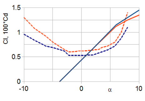
The significant aerodynamic properties of aircraft wings are summarised by two dimensionless quantities, the lift and drag coefficients C_L and C_D. Like other such aerodynamic quantities, they are functions only of the angle of attack α, the Reynolds number R_e and the Mach number M. C_L and C_D are often presented individually, plotted against α, but an alternative graph plots C_L as a function of C_D, using α parametrically.^[1][2] Similar plots can be made for other components or for whole aircraft; in all cases they are referred to as drag polars. The drag polar of an aircraft contains almost all the information required to analyse its performance and hence to begin a design.^[1]

Since the lift and the drag forces, L and D are scaled by the same factor to get C_L and C_D, L/D = C_L/C_D. As L and D are at right angles, the latter parallel to the free stream velocity or relative velocity of the surrounding, distant, air, the resultant force R lies at the same angle to that direction as the line from the origin of the polar plot to the corresponding C_L, C_D point does to the C_D axis. If, in a wind tunnel or whirling arm system an aerodynamic surface is held at a fixed angle of attack and both the magnitude and direction of the resulting force measured, they can be plotted using polar coordinates. When this measurement is repeated at different angles of attack the drag polar is obtained. Lift and drag data was gathered in this way in the 1880s by Otto Lilienthal and around 1910 by Gustav Eiffel, though not presented in terms of the more recent coefficients. Eiffel was the first to use the name drag polar.^[1]

Because of the Reynolds and Mach number dependence of the coefficients, families of drag polars may be plotted together. The design of a fighter will involve a set at different Mach numbers, whereas gliders, which spend their time either flying slowly in thermals or rapidly between them may require polars at different Reynolds numbers but are unaffected by compressibility effects. During the evolution of the design the drag polar will be refined. A particular aircraft may have different polar plots even at the same R_e and M values, depending for example on whether undercarriage and flaps are deployed.^[1]

Drag polar for light aircraft. C_D0= 0.017, K = 0.075 and C_L0 = 0.1. The tangent gives the maximum L/D point. https://handwiki.org/wiki/index.php?curid=1905922

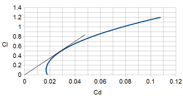
The accompanying diagram shows a drag polar for a typical light aircraft. Such diagrams identify a minimum C_D point at the left-most point on the plot, where the drag is locally independent of lift; to the right, the drag is lift related. One component here is the induced drag of the wing, an unavoidable companion of the wing's lift, though one that can be reduced by increasing the aspect ratio. Prandtl's lifting line theoretical work shows that this increases as C_L². The other drag mechanisms, parasitic and wave drag, have both constant components, totalling C_D0 say, and C_L dependent contributions that are often assumed to increase as C_L². If so, then

C_D = C_D0 + K.(C_L - C_L0)².

The effect of C_L0 is to lift the polar curve upwards; physically this is caused by some vertical asymmetry, such as a cambered wing or a finite angle of incidence, which ensures the minimum drag attitude produces lift and increases the maximum lift to drag ratio.^[1][3]

2. Power Required Plots

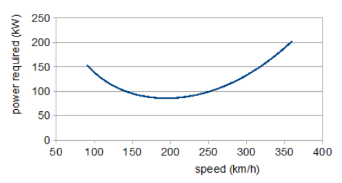
One example of the way the polar is used in the design process is the calculation of the power required (P_R) curve, which plots the power needed for steady, level flight over the operating speed range. The forces involved are obtained from the coefficients by multiplication with (ρ/2).S V², where ρ is the density of the atmosphere at the flight altitude, S is the wing area and V is the speed. In level flight, lift equals weight W and thrust equals drag, so

P_R curve for the light aircraft with the drag polar above and weighing 2000 kg, with a wing area of 15 m² and a propeller efficiency of 0.8.

W = (ρ/2).S.V².C_L and

P_R = (ρ/2η).S.V³.C_D.

The extra factor of V/η, with η the propeller efficiency, in the second equation enters because P_R= (required thrust)×V/η. Power rather than thrust is appropriate for a propeller driven aircraft, since it is roughly independent of speed; jet engines produce constant thrust. Since the weight is constant, the first of these equations determines how C_L falls with increasing speed. Putting these C_L values into the second equation with C_D from the drag polar produces the power curve. The low speed region shows a fall in lift induced drag, through a minimum followed by an increase in profile drag at higher speeds. The minimum power required, at a speed of 195 km/h  (121 mph) is about 86 kW (115 hp); 135 kW (181 hp) is required for a maximum speed of 300 km/h (186 mph). Flight at the power minimum will provide maximum endurance; the speed for greatest range is where the tangent to the power curve passes through the origin, about 240 km/h (150 mph).^[4])

If an analytical expression for the polar is available, useful relationships can be developed by differentiation. For example the form above, simplified slightly by putting C_L0 = 0, has a maximum C_L/C_D at C_L² = C_D0/K. For a propeller aircraft this is the maximum endurance condition and gives a speed of 185 km/h (115 mph). The corresponding maximum range condition is the maximum of C_L^3/2/C_D, at C_L² = 3.C_D0/K, and so the optimum speed is 244 km/h (152 mph). The effects of the approximation C_L0 = 0 are less than 5%; of course, with a finite C_L0 = 0.1, the analytic and graphical methods give the same results.^[4]

3. Rate of Climb

For an aircraft to climb at an angle θ and at speed V its engine must be developing more power, P say, than that P_R required to balance the drag experienced at that speed in level flight and shown on the power required plot. In level flight P_R/V = D but in the climb there is the additional weight component to include, that is

P/V = D + W.sin θ = P_R/V + W.sin θ.

Hence the climb rate RC = V.sin θ = (P - P_R)/W.^[5] Supposing the 135 kW engine required for a maximum speed at 300 km/h is fitted, the maximum excess power is 135 - 87 = 48 Kw at the minimum of P_R and the rate of climb 2.4 m/s. This suggests a more powerful engine is called for.

4. Glider Polars

The same aircraft, without power. The tangent defines the minimum glide angle. https://handwiki.org/wiki/index.php?curid=1615890

Without power, a gliding aircraft has only gravity to propel it. At a glide angle of θ, the weight has two components, W.cos θ at right angles to the flight line and W.sin θ parallel to it. These are balanced by the force and lift components respectively, so

W.cos θ = (ρ/2).S.V².C_L and

W. sin θ = (ρ/2).S.V².C_D.

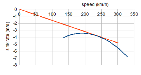
Dividing one equation by the other shows that the glide angle is given by tan θ = C_D/C_L. The performance characteristics of most interest in unpowered flight are the speed across the ground, V_g say, and the sink speed V_s; these are displayed by plotting V.sin θ = V_s against V.cos θ = V_g. Such plots are generally termed polars, and to produce them the glide angle as a function of V is required.^[6]

One way of finding solutions to the two force equations is to square them both then add together; this shows the possible C_L, C_D values lie on a circle of radius 2.W / S.ρ.V². When this is plotted on the drag polar, the intersection of the two curves locates the solution and its θ value read off. Alternatively, bearing in mind that glides are usually shallow, the approximation cos θ ≃ 1, good for θ less than 10°, can be used in the lift equation and the value of C_L for a chosen V calculated, finding C_L from the drag polar and then calculating θ.^[6]

The example polar here shows the gliding performance of the aircraft analysed above, assuming its drag polar is not much altered by the stationary propeller. A straight line from the origin to some point on the curve has a gradient equal to the glide angle at that speed, so the corresponding tangent shows the best glide angle tan⁻¹(C_D/C_L)_min ≃ 3.3°. This is not the lowest rate of sink but provides the greatest range, requiring a speed of 240  km/h (149 mph); the minimum sink rate of about 3.5 m/s is at 180 km/h (112 mph), speeds seen in the previous, powered plots.^[6]

References

- Anderson, John D. Jnr. (1999). Aircraft Performance and Design. Cambridge: WCB/McGraw-Hill. ISBN 0-07-116010-8.
- Abbott, Ira H.; von Doenhoff, Albert E. (1958). Theory of wing sections. New York: Dover Publications. pp. 57–70;129–142. ISBN 0-486-60586-8.
- Aircraft Performance and Design. pp. 414–5.
- Aircraft Performance and Design. pp. 199–252, 293–309.
- Aircraft Performance and Design. pp. 265–270.
- Aircraft Performance and Design. pp. 282–7.