 +1 credit
| Version | Summary | Created by | Modification | Content Size | Created at | Operation |
|---|---|---|---|---|---|---|
| 1 | Camila Xu | -- | 7237 | 2022-10-19 01:32:31 |
Video Upload Options
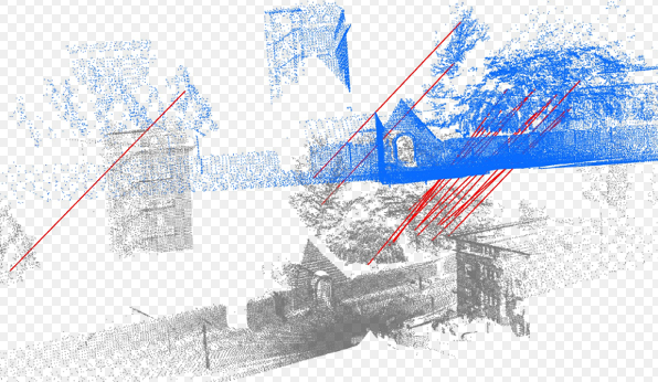
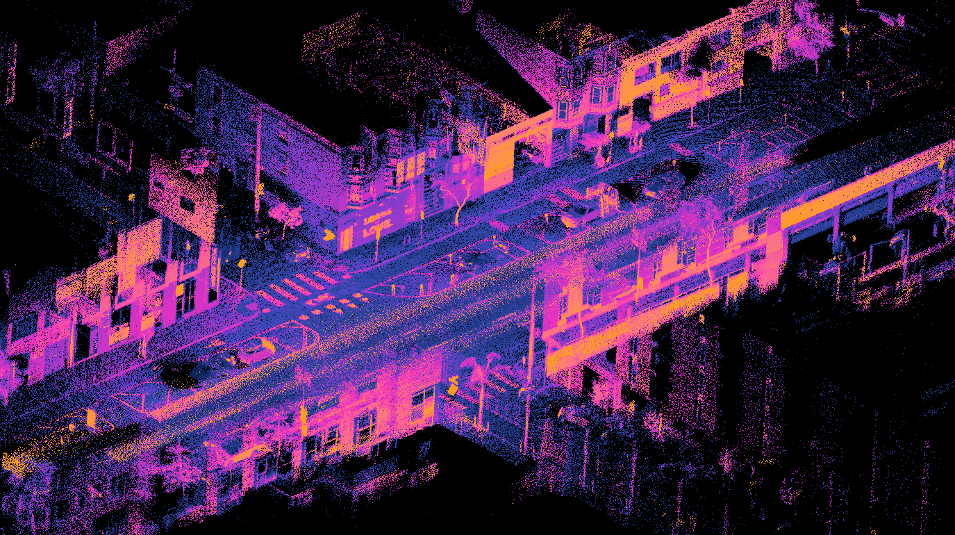
In computer vision, pattern recognition, and robotics, point set registration, also known as point cloud registration or scan matching, is the process of finding a spatial transformation (e.g., scaling, rotation and translation) that aligns two point clouds. The purpose of finding such a transformation includes merging multiple data sets into a globally consistent model (or coordinate frame), and mapping a new measurement to a known data set to identify features or to estimate its pose. Raw 3D point cloud data are typically obtained from Lidars and RGB-D cameras. 3D point clouds can also be generated from computer vision algorithms such as triangulation, bundle adjustment, and more recently, monocular image depth estimation using deep learning. For 2D point set registration used in image processing and feature-based image registration, a point set may be 2D pixel coordinates obtained by feature extraction from an image, for example corner detection. Point cloud registration has extensive applications in autonomous driving, motion estimation and 3D reconstruction, object detection and pose estimation, robotic manipulation, simultaneous localization and mapping (SLAM), panorama stitching, virtual and augmented reality, and medical imaging. As a special case, registration of two point sets that only differ by a 3D rotation (i.e., there is no scaling and translation), is called the Wahba Problem and also related to the orthogonal procrustes problem.
1. Formulation

The problem may be summarized as follows:[1] Let [math]\displaystyle{ \lbrace\mathcal{M},\mathcal{S}\rbrace }[/math] be two finite size point sets in a finite-dimensional real vector space [math]\displaystyle{ \mathbb{R}^d }[/math], which contain [math]\displaystyle{ M }[/math] and [math]\displaystyle{ N }[/math] points respectively (e.g., [math]\displaystyle{ d=3 }[/math] recovers the typical case of when [math]\displaystyle{ \mathcal{M} }[/math] and [math]\displaystyle{ \mathcal{S} }[/math] are 3D point sets). The problem is to find a transformation to be applied to the moving "model" point set [math]\displaystyle{ \mathcal{M} }[/math] such that the difference (typically defined in the sense of point-wise Euclidean distance) between [math]\displaystyle{ \mathcal{M} }[/math] and the static "scene" set [math]\displaystyle{ \mathcal{S} }[/math] is minimized. In other words, a mapping from [math]\displaystyle{ \mathbb{R}^d }[/math] to [math]\displaystyle{ \mathbb{R}^d }[/math] is desired which yields the best alignment between the transformed "model" set and the "scene" set. The mapping may consist of a rigid or non-rigid transformation. The transformation model may be written as [math]\displaystyle{ T }[/math], using which the transformed, registered model point set is:
-
[math]\displaystyle{ T(\mathcal{M}) }[/math]
()
The output of a point set registration algorithm is therefore the optimal transformation [math]\displaystyle{ T^\star }[/math] such that [math]\displaystyle{ \mathcal{M} }[/math] is best aligned to [math]\displaystyle{ \mathcal{S} }[/math], according to some defined notion of distance function [math]\displaystyle{ \operatorname{dist}(\cdot,\cdot) }[/math]:
-
[math]\displaystyle{ T^\star = \arg\min_{T \in \mathcal{T} } \text{dist}(T(\mathcal{M}),\mathcal{S}) }[/math]
()
where [math]\displaystyle{ \mathcal{T} }[/math] is used to denote the set of all possible transformations that the optimization tries to search for. The most popular choice of the distance function is to take the square of the Euclidean distance for every pair of points:
-
[math]\displaystyle{ \operatorname{dist}(T(\mathcal{M}), \mathcal{S}) = \sum_{m \in T(\mathcal{M})} \Vert m - s_m \Vert^2_2, \quad s_m = \arg\min_{s \in \mathcal{S} } \Vert s - m \Vert_2^2 }[/math]
()
where [math]\displaystyle{ \| \cdot \|_2 }[/math] denotes the vector 2-norm, [math]\displaystyle{ s_m }[/math] is the corresponding point in set [math]\displaystyle{ \mathcal{S} }[/math] that attains the shortest distance to a given point [math]\displaystyle{ m }[/math] in set [math]\displaystyle{ \mathcal{M} }[/math] after transformation. Minimizing such a function in rigid registration is equivalent to solving a least squares problem.
2. Types of Algorithms
When the correspondences (i.e., [math]\displaystyle{ s_m \leftrightarrow m }[/math]) are given before the optimization, for example, using feature matching techniques, then the optimization only needs to estimate the transformation. This type of registration is called correspondence-based registration. On the other hand, if the correspondences are unknown, then the optimization is required to jointly find out the correspondences and transformation together. This type of registration is called simultaneous pose and correspondence registration.
2.1. Rigid Registration
Given two point sets, rigid registration yields a rigid transformation which maps one point set to the other. A rigid transformation is defined as a transformation that does not change the distance between any two points. Typically such a transformation consists of translation and rotation.[2] In rare cases, the point set may also be mirrored. In robotics and computer vision, rigid registration has the most applications.
2.2. Non-Rigid Registration
Given two point sets, non-rigid registration yields a non-rigid transformation which maps one point set to the other. Non-rigid transformations include affine transformations such as scaling and shear mapping. However, in the context of point set registration, non-rigid registration typically involves nonlinear transformation. If the eigenmodes of variation of the point set are known, the nonlinear transformation may be parametrized by the eigenvalues.[3] A nonlinear transformation may also be parametrized as a thin plate spline.[3][4]
2.3. Other Types
Some approaches to point set registration use algorithms that solve the more general graph matching problem.[1] However, the computational complexity of such methods tend to be high and they are limited to rigid registrations. In this article, we will only consider algorithms for rigid registration, where the transformation is assumed to contain 3D rotations and translations (possibly also including a uniform scaling).
The PCL (Point Cloud Library) is an open-source framework for n-dimensional point cloud and 3D geometry processing. It includes several point registration algorithms.[5]
3. Correspondence-based Registration
Correspondence-based methods assume the putative correspondences [math]\displaystyle{ m \leftrightarrow s_m }[/math] are given for every point [math]\displaystyle{ m \in \mathcal{M} }[/math]. Therefore, we arrive at a setting where both point sets [math]\displaystyle{ \mathcal{M} }[/math] and [math]\displaystyle{ \mathcal{S} }[/math] have [math]\displaystyle{ N }[/math] points and the correspondences [math]\displaystyle{ m_i \leftrightarrow s_i,i=1,\dots,N }[/math]are given.
3.1. Outlier-Free Registration
In the simplest case, one can assume that all the correspondences are correct, meaning that the points [math]\displaystyle{ m_i,s_i \in \mathbb{R}^3 }[/math] are generated as follows:
-
[math]\displaystyle{ s_i = lR m_i + t + \epsilon_i, i=1,\dots,N }[/math]
()
where [math]\displaystyle{ l \gt 0 }[/math] is a uniform scaling factor (in many cases [math]\displaystyle{ l=1 }[/math] is assumed), [math]\displaystyle{ R \in \text{SO}(3) }[/math] is a proper 3D rotation matrix ([math]\displaystyle{ \text{SO}(d) }[/math] is the special orthogonal group of degree [math]\displaystyle{ d }[/math]), [math]\displaystyle{ t \in \mathbb{R}^3 }[/math] is a 3D translation vector and [math]\displaystyle{ \epsilon_i \in \mathbb{R}^3 }[/math] models the unknown additive noise (e.g., Gaussian noise). Specifically, if the noise [math]\displaystyle{ \epsilon_i }[/math] is assumed to follow a zero-mean isotropic Gaussian distribution with standard deviation [math]\displaystyle{ \sigma_i }[/math], i.e., [math]\displaystyle{ \epsilon_i \sim \mathcal{N}(0,\sigma_i^2 I_3 ) }[/math], then the following optimization can be shown to yield the maximum likelihood estimate for the unknown scale, rotation and translation:
-
[math]\displaystyle{ l^\star, R^\star, t^\star = \arg\min_{l\gt 0, R \in \text{SO}(3), t \in \mathbb{R}^3} \sum_{i=1}^N \frac{1}{\sigma_i^2} \left\Vert s_i - lRm_i - t \right\Vert_2^2 }[/math]
()
Note that when the scaling factor is 1 and the translation vector is zero, then the optimization recovers the formulation of the Wahba problem. Despite the non-convexity of the optimization (cb.2) due to non-convexity of the set [math]\displaystyle{ \text{SO}(3) }[/math], seminal work by Berthold K.P. Horn showed that (cb.2) actually admits a closed-form solution, by decoupling the estimation of scale, rotation and translation.[6] Similar results were discovered by Arun et al.[7] In addition, in order to find a unique transformation [math]\displaystyle{ (l,R,t) }[/math], at least [math]\displaystyle{ N=3 }[/math] non-collinear points in each point set are required.
More recently, Briales and Gonzalez-Jimenez have developed a semidefinite relaxation using Lagrangian duality, for the case where the model set [math]\displaystyle{ \mathcal{M} }[/math] contains different 3D primitives such as points, lines and planes (which is the case when the model [math]\displaystyle{ \mathcal{M} }[/math] is a 3D mesh).[8] Interestingly, the semidefinite relaxation is empirically tight, i.e., a certifiably globally optimal solution can be extracted from the solution of the semidefinite relaxation.
3.2. Robust Registration
The least squares formulation (cb.2) is known to perform arbitrarily bad in the presence of outliers. An outlier correspondence is a pair of measurements [math]\displaystyle{ s_i \leftrightarrow m_i }[/math] that departs from the generative model (cb.1). In this case, one can consider a different generative model as follows:[9]
-
[math]\displaystyle{ s_i = \begin{cases} l R m_i + t + \epsilon_i & \text{if } i- \text{th pair is an inlier} \\ o_i & \text{if } i- \text{th pair is an outlier} \end{cases} }[/math]
()
where if the [math]\displaystyle{ i- }[/math]th pair [math]\displaystyle{ s_i \leftrightarrow m_i }[/math] is an inlier, then it obeys the outlier-free model (cb.1), i.e., [math]\displaystyle{ s_i }[/math] is obtained from [math]\displaystyle{ m_i }[/math] by a spatial transformation plus some small noise; however, if the [math]\displaystyle{ i- }[/math]th pair [math]\displaystyle{ s_i \leftrightarrow m_i }[/math] is an outlier, then [math]\displaystyle{ s_i }[/math] can be any arbitrary vector [math]\displaystyle{ o_i }[/math]. Since one does not know which correspondences are outliers beforehand, robust registration under the generative model (cb.3) is of paramount importance for computer vision and robotics deployed in the real world, because current feature matching techniques tend to output highly corrupted correspondences where over [math]\displaystyle{ 95\% }[/math] of the correspondences can be outliers.[10]
Next, we describe several common paradigms for robust registration.
Maximum consensus
Maximum consensus seeks to find the largest set of correspondences that are consistent with the generative model (cb.1) for some choice of spatial transformation [math]\displaystyle{ (l,R,t) }[/math]. Formally speaking, maximum consensus solves the following optimization:
-
[math]\displaystyle{ \max_{l\gt 0,R \in \text{SO}(3), t \in \mathbb{R}^3, \mathcal{I} } \vert \mathcal{I} \vert, \quad \text{subject to } \frac{1}{\sigma_i^2} \Vert s_i - lRm_i - t\Vert_2^2 \leq \xi, \forall i \in \mathcal{I} }[/math]
()
where [math]\displaystyle{ \vert \mathcal{I} \vert }[/math] denotes the cardinality of the set [math]\displaystyle{ \mathcal{I} }[/math]. The constraint in (cb.4) enforces that every pair of measurements in the inlier set [math]\displaystyle{ \mathcal{I} }[/math] must have residuals smaller than a pre-defined threshold [math]\displaystyle{ \xi }[/math]. Unfortunately, recent analyses have shown that globally solving problem (cb.4) is NP-Hard, and global algorithms typically have to resort to branch-and-bound (BnB) techniques that take exponential-time complexity in the worst case.[11][12][13][14][15]
Although solving consensus maximization exactly is hard, there exist efficient heuristics that perform quite well in practice. One of the most popular heuristics is the Random Sample Consensus (RANSAC) scheme.[16] RANSAC is an iterative hypothesize-and-verity method. At each iteration, the method first randomly samples 3 out of the total number of [math]\displaystyle{ N }[/math] correspondences and computes a hypothesis [math]\displaystyle{ (l,R,t) }[/math] using Horn's method,[6] then the method evaluates the constraints in (cb.4) to count how many correspondences actually agree with such a hypothesis (i.e., it computes the residual [math]\displaystyle{ \Vert s_i - lRm_i - t \Vert_2^2 / \sigma_i^2 }[/math] and compares it with the threshold [math]\displaystyle{ \xi }[/math] for each pair of measurements). The algorithm terminates either after it has found a consensus set that has enough correspondences, or after it has reached the total number of allowed iterations. RANSAC is highly efficient because the main computation of each iteration is carrying out the closed-form solution in Horn's method. However, RANSAC is non-deterministic and only works well in the low-outlier-ratio regime (e.g., below [math]\displaystyle{ 50\% }[/math]), because its runtime grows exponentially with respect to the outlier ratio.[10]
To fill the gap between the fast but inexact RANSAC scheme and the exact but exhaustive BnB optimization, recent researches have developed deterministic approximate methods to solve consensus maximization.[11][12][13][17]
Outlier removal
Outlier removal methods seek to pre-process the set of highly corrupted correspondences before estimating the spatial transformation. The motivation of outlier removal is to significantly reduce the number of outlier correspondences, while maintaining inlier correspondences, so that optimization over the transformation becomes easier and more efficient (e.g., RANSAC works poorly when the outlier ratio is above [math]\displaystyle{ 95\% }[/math] but performs quite well when outlier ratio is below [math]\displaystyle{ 50\% }[/math]).
Parra et al. have proposed a method called Guaranteed Outlier Removal (GORE) that uses geometric constraints to prune outlier correspondences while guaranteeing to preserve inlier correspondences.[10] GORE has been shown to be able to drastically reduce the outlier ratio, which can significantly boost the performance of consensus maximization using RANSAC or BnB. Yang and Carlone have proposed to build pairwise translation-and-rotation-invariant measurements (TRIMs) from the original set of measurements and embed TRIMs as the edges of a graph whose nodes are the 3D points. Since inliers are pairwise consistent in terms of the scale, they must form a clique within the graph. Therefore, using efficient algorithms for computing the maximum clique of a graph can find the inliers and effectively prune the outliers.[18] The maximum clique based outlier removal method is also shown to be quite useful in real-world point set registration problems.[9] Similar outlier removal ideas were also proposed by Parra et al..[19]
M-estimation
M-estimation replaces the least squares objective function in (cb.2) with a robust cost function that is less sensitive to outliers. Formally, M-estimation seeks to solve the following problem:
-
[math]\displaystyle{ l^\star, R^\star, t^\star = \arg\min_{l\gt 0, R \in \text{SO}(3), t \in \mathbb{R}^3} \sum_{i=1}^N \rho\left( \frac{1}{\sigma_i} \left\Vert s_i - lRm_i - t \right\Vert_2 \right) }[/math]
()
where [math]\displaystyle{ \rho(\cdot) }[/math] represents the choice of the robust cost function. Note that choosing [math]\displaystyle{ \rho(x) = x^2 }[/math] recovers the least squares estimation in (cb.2). Popular robust cost functions include [math]\displaystyle{ \ell_1 }[/math]-norm loss, Huber loss,[20] Geman-McClure loss[21] and truncated least squares loss.[9][18][22] M-estimation has been one of the most popular paradigms for robust estimation in robotics and computer vision.[23][24] Because robust objective functions are typically non-convex (e.g., the truncated least squares loss v.s. the least squares loss), algorithms for solving the non-convex M-estimation are typically based on local optimization, where first an initial guess is provided, following by iterative refinements of the transformation to keep decreasing the objective function. Local optimization tends to work well when the initial guess is close to the global minimum, but it is also prone to get stuck in local minima if provided with poor initialization.
Graduated non-convexity
Graduated non-convexity (GNC) is a general-purpose framework for solving non-convex optimization problems without initialization. It has achieved success in early vision and machine learning applications.[25][26] The key idea behind GNC is to solve the hard non-convex problem by starting from an easy convex problem. Specifically, for a given robust cost function [math]\displaystyle{ \rho(\cdot) }[/math], one can construct a surrogate function [math]\displaystyle{ \rho_{\mu}(\cdot) }[/math] with a hyper-parameter [math]\displaystyle{ \mu }[/math], tuning which can gradually increase the non-convexity of the surrogate function [math]\displaystyle{ \rho_{\mu}(\cdot) }[/math] until it converges to the target function [math]\displaystyle{ \rho(\cdot) }[/math].[26][27] Therefore, at each level of the hyper-parameter [math]\displaystyle{ \mu }[/math], the following optimization is solved:
-
[math]\displaystyle{ l_{\mu}^\star, R_{\mu}^\star, t_{\mu}^\star = \arg\min_{l\gt 0, R \in \text{SO}(3), t \in \mathbb{R}^3} \sum_{i=1}^N \rho_{\mu}\left( \frac{1}{\sigma_i} \left\Vert s_i - l Rm_i - t \right\Vert_2 \right) }[/math]
()
Black and Rangarajan proved that the objective function of each optimization (cb.6) can be dualized into a sum of weighted least squares and a so-called outlier process function on the weights that determine the confidence of the optimization in each pair of measurements.[25] Using Black-Rangarajan duality and GNC tailored for the Geman-McClure function, Zhou et al. developed the fast global registration algorithm that is robust against about [math]\displaystyle{ 80\% }[/math] outliers in the correspondences.[21] More recently, Yang et al. showed that the joint use of GNC (tailored to the Geman-McClure function and the truncated least squares function) and Black-Rangarajan duality can lead to a general-purpose solver for robust registration problems, including point clouds and mesh registration.[27]
Certifiably robust registration
Almost none of the robust registration algorithms mentioned above (except the BnB algorithm that runs in exponential-time in the worst case) comes with performance guarantees, which means that these algorithms can return completely incorrect estimates without notice. Therefore, these algorithms are undesirable for safety-critical applications like autonomous driving.
Very recently, Yang et al. has developed the first certifiably robust registration algorithm, named Truncated least squares Estimation And SEmidefinite Relaxation (TEASER).[9] For point cloud registration, TEASER not only outputs an estimate of the transformation, but also quantifies the optimality of the given estimate. TEASER adopts the following truncated least squares (TLS) estimator:
-
[math]\displaystyle{ l^\star, R^\star, t^\star = \arg\min_{l \gt 0, R \in \text{SO}(3), t \in \mathbb{R}^3} \sum_{i=1}^N \min \left( \frac{1}{\sigma_i^2} \left\Vert s_i - l Rm_i - t \right\Vert_2^2, \bar{c}^2 \right) }[/math]
()
which is obtained by choosing the TLS robust cost function [math]\displaystyle{ \rho(x) = \min (x^2, \bar{c}^2) }[/math], where [math]\displaystyle{ \bar{c}^2 }[/math]is a pre-defined constant that determines the maximum allowed residuals to be considered inliers. The TLS objective function has the property that for inlier correspondences ([math]\displaystyle{ \Vert s_i - l Rm_i - t \Vert_2^2 / \sigma_i^2 \lt \bar{c}^2 }[/math]), the usual least square penalty is applied; while for outlier correspondences ([math]\displaystyle{ \Vert s_i - l Rm_i - t \Vert_2^2 / \sigma_i^2 \gt \bar{c}^2 }[/math]), no penalty is applied and the outliers are discarded. If the TLS optimization (cb.7) is solved to global optimality, then it is equivalent to running Horn's method on only the inlier correspondences.
However, solving (cb.7) is quite challenging due to its combinatorial nature. TEASER solves (cb.7) as follows : (i) It builds invariant measurements such that the estimation of scale, rotation and translation can be decoupled and solved separately, a strategy that is inspired by the original Horn's method; (ii) The same TLS estimation is applied for each of the three sub-problems, where the scale TLS problem can be solved exactly using an algorithm called adaptive voting, the rotation TLS problem can relaxed to a semidefinite program (SDP) where the relaxation is exact in practice,[22] even with large amount of outliers; the translation TLS problem can solved using component-wise adaptive voting. A fast implementation leveraging GNC is open-sourced here. In practice, TEASER can tolerate more than [math]\displaystyle{ 99\% }[/math] outlier correspondences and runs in milliseconds.
In addition to developing TEASER, Yang et al. also prove that, under some mild conditions on the point cloud data, TEASER's estimated transformation has bounded errors from the ground-truth transformation.[9]
4. Simultaneous Pose and Correspondence Registration
4.1. Iterative Closest Point
The iterative closest point (ICP) algorithm was introduced by Besl and McKay.[28] The algorithm performs rigid registration in an iterative fashion by alternating in (i) given the transformation, finding the closest point in [math]\displaystyle{ \mathcal{S} }[/math] for every point in [math]\displaystyle{ \mathcal{M} }[/math]; and (ii) given the correspondences, finding the best rigid transformation by solving the least squares problem (cb.2). As such, it works best if the initial pose of [math]\displaystyle{ \mathcal{M} }[/math] is sufficiently close to [math]\displaystyle{ \mathcal{S} }[/math]. In pseudocode, the basic algorithm is implemented as follows:
algorithm ICP(M, S) θ := θ0 while not registered: X := ∅ for mi ∊ T(M, θ): ŝj := closest point in S to mi X := X + ⟨mi, ŝj⟩ θ := least_squares(X) return θ
Here, the function least_squares performs least squares optimization to minimize the distance in each of the [math]\displaystyle{ \langle m_i, \hat{s}_j \rangle }[/math] pairs, using the closed-form solutions by Horn[6] and Arun.[7]
Because the cost function of registration depends on finding the closest point in [math]\displaystyle{ \mathcal{S} }[/math] to every point in [math]\displaystyle{ \mathcal{M} }[/math], it can change as the algorithm is running. As such, it is difficult to prove that ICP will in fact converge exactly to the local optimum.[29] In fact, empirically, ICP and EM-ICP do not converge to the local minimum of the cost function.[29] Nonetheless, because ICP is intuitive to understand and straightforward to implement, it remains the most commonly used point set registration algorithm.[29] Many variants of ICP have been proposed, affecting all phases of the algorithm from the selection and matching of points to the minimization strategy.[3][30] For example, the expectation maximization algorithm is applied to the ICP algorithm to form the EM-ICP method, and the Levenberg-Marquardt algorithm is applied to the ICP algorithm to form the LM-ICP method.[2]
4.2. Robust Point Matching
Robust point matching (RPM) was introduced by Gold et al.[31] The method performs registration using deterministic annealing and soft assignment of correspondences between point sets. Whereas in ICP the correspondence generated by the nearest-neighbour heuristic is binary, RPM uses a soft correspondence where the correspondence between any two points can be anywhere from 0 to 1, although it ultimately converges to either 0 or 1. The correspondences found in RPM is always one-to-one, which is not always the case in ICP.[4] Let [math]\displaystyle{ m_i }[/math] be the [math]\displaystyle{ i }[/math]th point in [math]\displaystyle{ \mathcal{M} }[/math] and [math]\displaystyle{ s_j }[/math] be the [math]\displaystyle{ j }[/math]th point in [math]\displaystyle{ \mathcal{S} }[/math]. The match matrix [math]\displaystyle{ \mathbf{\mu} }[/math] is defined as such:
-
[math]\displaystyle{ \mu_{ij} = \begin{cases} 1 & \text{if point }m_i\text{ corresponds to point }s_j\\ 0 & \text{otherwise} \end{cases} }[/math]
()
The problem is then defined as: Given two point sets [math]\displaystyle{ \mathcal{M} }[/math] and [math]\displaystyle{ \mathcal{S} }[/math] find the Affine transformation [math]\displaystyle{ T }[/math] and the match matrix [math]\displaystyle{ \mathbf{\mu} }[/math] that best relates them.[31] Knowing the optimal transformation makes it easy to determine the match matrix, and vice versa. However, the RPM algorithm determines both simultaneously. The transformation may be decomposed into a translation vector and a transformation matrix:
- [math]\displaystyle{ T(m) = \mathbf{A}m + \mathbf{t} }[/math]
The matrix [math]\displaystyle{ \mathbf{A} }[/math] in 2D is composed of four separate parameters [math]\displaystyle{ \lbrace a, \theta, b, c\rbrace }[/math], which are scale, rotation, and the vertical and horizontal shear components respectively. The cost function is then:
-
[math]\displaystyle{ \operatorname{cost} = \sum_{j=1}^N \sum_{i=1}^M \mu_{ij} \lVert s_j - \mathbf{t} - \mathbf{A} m_i \rVert^2 + g(\mathbf{A}) - \alpha \sum_{j=1}^N \sum_{i=1}^M \mu_{ij} }[/math]
()
subject to [math]\displaystyle{ \forall j~\sum_{i=1}^M \mu_{ij} \leq 1 }[/math], [math]\displaystyle{ \forall i~\sum_{j=1}^N \mu_{ij} \leq 1 }[/math], [math]\displaystyle{ \forall ij~\mu_{ij} \in \lbrace0, 1\rbrace }[/math]. The [math]\displaystyle{ \alpha }[/math] term biases the objective towards stronger correlation by decreasing the cost if the match matrix has more ones in it. The function [math]\displaystyle{ g(\mathbf{A}) }[/math] serves to regularize the Affine transformation by penalizing large values of the scale and shear components:
- [math]\displaystyle{ g(\mathbf{A}(a,\theta, b, c)) = \gamma(a^2 + b^2 + c^2) }[/math]
for some regularization parameter [math]\displaystyle{ \gamma }[/math].
The RPM method optimizes the cost function using the Softassign algorithm. The 1D case will be derived here. Given a set of variables [math]\displaystyle{ \lbrace Q_j\rbrace }[/math] where [math]\displaystyle{ Q_j\in \mathbb{R}^1 }[/math]. A variable [math]\displaystyle{ \mu_j }[/math] is associated with each [math]\displaystyle{ Q_j }[/math] such that [math]\displaystyle{ \sum_{j=1}^J \mu_j = 1 }[/math]. The goal is to find [math]\displaystyle{ \mathbf{\mu} }[/math] that maximizes [math]\displaystyle{ \sum_{j=1}^J \mu_j Q_j }[/math]. This can be formulated as a continuous problem by introducing a control parameter [math]\displaystyle{ \beta \gt 0 }[/math]. In the deterministic annealing method, the control parameter [math]\displaystyle{ \beta }[/math] is slowly increased as the algorithm runs. Let [math]\displaystyle{ \mathbf{\mu} }[/math] be:
-
[math]\displaystyle{ \mu_{\hat{j}} = \frac{\exp{(\beta Q_{\hat{j}})}}{\sum_{j=1}^J \exp{(\beta Q_j)}} }[/math]
()
this is known as the softmax function. As [math]\displaystyle{ \beta }[/math] increases, it approaches a binary value as desired in Equation (rpm.1). The problem may now be generalized to the 2D case, where instead of maximizing [math]\displaystyle{ \sum_{j=1}^J \mu_j Q_j }[/math], the following is maximized:
-
[math]\displaystyle{ E(\mu) = \sum_{j=1}^N \sum_{i=0}^M \mu_{ij} Q_{ij} }[/math]
()
where
- [math]\displaystyle{ Q_{ij} = -(\lVert s_j - \mathbf{t} - \mathbf{A} m_i \rVert^2 - \alpha) = -\frac{\partial \operatorname{cost}}{\partial \mu_{ij}} }[/math]
This is straightforward, except that now the constraints on [math]\displaystyle{ \mu }[/math] are doubly stochastic matrix constraints: [math]\displaystyle{ \forall j~\sum_{i=1}^M \mu_{ij} = 1 }[/math] and [math]\displaystyle{ \forall i~\sum_{j=1}^N \mu_{ij} = 1 }[/math]. As such the denominator from Equation (rpm.3) cannot be expressed for the 2D case simply. To satisfy the constraints, it is possible to use a result due to Sinkhorn,[31] which states that a doubly stochastic matrix is obtained from any square matrix with all positive entries by the iterative process of alternating row and column normalizations. Thus the algorithm is written as such:[31]
algorithm RPM2D[math]\displaystyle{ (\mathcal{M}, \mathcal{S}) }[/math] t := 0 a, θ b, c := 0 β := β0 [math]\displaystyle{ \hat{\mu}_{ij} := 1 + \epsilon }[/math] while β < βf: while μ has not converged: // update correspondence parameters by softassign [math]\displaystyle{ Q_{ij} := -\frac{\partial \operatorname{cost}}{\partial \mu_{ij}} }[/math] [math]\displaystyle{ \mu^0_{ij} := \exp(\beta Q_{ij}) }[/math] // apply Sinkhorn's method while [math]\displaystyle{ \hat{\mu} }[/math] has not converged: // update [math]\displaystyle{ \hat{\mu} }[/math] by normalizing across all rows: [math]\displaystyle{ \hat{\mu}^1_{ij} := \frac{\hat{\mu}^0_{ij}}{\sum_{i=1}^{M+1} \hat{\mu}^0_{ij}} }[/math] // update [math]\displaystyle{ \hat{\mu} }[/math] by normalizing across all columns: [math]\displaystyle{ \hat{\mu}^0_{ij} := \frac{\hat{\mu}^1_{ij}}{\sum_{j=1}^{N+1} \hat{\mu}^1_{ij}} }[/math] // update pose parameters by coordinate descent update θ using analytical solution update t using analytical solution update a, b, c using Newton's method [math]\displaystyle{ \beta := \beta_r \beta }[/math] [math]\displaystyle{ \gamma := \frac{\gamma}{\beta_r} }[/math] return a, b, c, θ and t
where the deterministic annealing control parameter [math]\displaystyle{ \beta }[/math] is initially set to [math]\displaystyle{ \beta_0 }[/math] and increases by factor [math]\displaystyle{ \beta_r }[/math] until it reaches the maximum value [math]\displaystyle{ \beta_f }[/math]. The summations in the normalization steps sum to [math]\displaystyle{ M+1 }[/math] and [math]\displaystyle{ N+1 }[/math] instead of just [math]\displaystyle{ M }[/math] and [math]\displaystyle{ N }[/math] because the constraints on [math]\displaystyle{ \mu }[/math] are inequalities. As such the [math]\displaystyle{ M+1 }[/math]th and [math]\displaystyle{ N+1 }[/math]th elements are slack variables.
The algorithm can also be extended for point sets in 3D or higher dimensions. The constraints on the correspondence matrix [math]\displaystyle{ \mathbf{\mu} }[/math] are the same in the 3D case as in the 2D case. Hence the structure of the algorithm remains unchanged, with the main difference being how the rotation and translation matrices are solved.[31]
Thin plate spline robust point matching
The thin plate spline robust point matching (TPS-RPM) algorithm by Chui and Rangarajan augments the RPM method to perform non-rigid registration by parametrizing the transformation as a thin plate spline.[4] However, because the thin plate spline parametrization only exists in three dimensions, the method cannot be extended to problems involving four or more dimensions.
4.3. Kernel Correlation
The kernel correlation (KC) approach of point set registration was introduced by Tsin and Kanade.[29] Compared with ICP, the KC algorithm is more robust against noisy data. Unlike ICP, where, for every model point, only the closest scene point is considered, here every scene point affects every model point.[29] As such this is a multiply-linked registration algorithm. For some kernel function [math]\displaystyle{ K }[/math], the kernel correlation [math]\displaystyle{ KC }[/math] of two points [math]\displaystyle{ x_i, x_j }[/math] is defined thus:[29]
-
[math]\displaystyle{ KC(x_i, x_j) = \int K(x, x_i) \cdot K(x, x_j) dx }[/math]
()
The kernel function [math]\displaystyle{ K }[/math] chosen for point set registration is typically symmetric and non-negative kernel, similar to the ones used in the Parzen window density estimation. The Gaussian kernel typically used for its simplicity, although other ones like the Epanechnikov kernel and the tricube kernel may be substituted.[29] The kernel correlation of an entire point set [math]\displaystyle{ \mathcal{\chi} }[/math] is defined as the sum of the kernel correlations of every point in the set to every other point in the set:[29]
-
[math]\displaystyle{ KC(\mathcal{X}) = \sum_{i\neq j}KC(x_i, x_j) = 2\sum_{i\lt j}KC(x_i, x_j) }[/math]
()
The logarithm of KC of a point set is proportional, within a constant factor, to the information entropy. Observe that the KC is a measure of a "compactness" of the point set—trivially, if all points in the point set were at the same location, the KC would evaluate to a large value. The cost function of the point set registration algorithm for some transformation parameter [math]\displaystyle{ \theta }[/math] is defined thus:
-
[math]\displaystyle{ \operatorname{cost}(\mathcal{S}, \mathcal{M}, \theta) = -\sum_{m \in \mathcal{M}} \sum_{s \in \mathcal{S}} KC(s, T(m, \theta)) }[/math]
()
Some algebraic manipulation yields:
-
[math]\displaystyle{ KC(\mathcal{S} \cup T(\mathcal{M}, \theta)) = KC(\mathcal{S}) + KC(T(\mathcal{M}, \theta)) - 2 \operatorname{cost}(\mathcal{S}, \mathcal{M}, \theta) }[/math]
()
The expression is simplified by observing that [math]\displaystyle{ KC(\mathcal{S}) }[/math] is independent of [math]\displaystyle{ \theta }[/math]. Furthermore, assuming rigid registration, [math]\displaystyle{ KC(T(\mathcal{M}, \theta)) }[/math] is invariant when [math]\displaystyle{ \theta }[/math] is changed because the Euclidean distance between every pair of points stays the same under rigid transformation. So the above equation may be rewritten as:
-
[math]\displaystyle{ KC(\mathcal{S} \cup T(\mathcal{M}, \theta)) = C - 2 \operatorname{cost}(\mathcal{S}, \mathcal{M}, \theta) }[/math]
()
The kernel density estimates are defined as:
- [math]\displaystyle{ P_{\mathcal{M}}(x, \theta) = \frac{1}{M} \sum_{m \in \mathcal{M}} K(x, T(m, \theta)) }[/math]
- [math]\displaystyle{ P_{\mathcal{S}}(x) = \frac{1}{N} \sum_{s \in \mathcal{S}} K(x, s) }[/math]
The cost function can then be shown to be the correlation of the two kernel density estimates:
-
[math]\displaystyle{ \operatorname{cost}(\mathcal{S}, \mathcal{M}, \theta) = -N^2 \int_x P_{\mathcal{M}}\cdot P_{\mathcal{S}} ~ dx }[/math]
()
Having established the cost function, the algorithm simply uses gradient descent to find the optimal transformation. It is computationally expensive to compute the cost function from scratch on every iteration, so a discrete version of the cost function Equation (kc.6) is used. The kernel density estimates [math]\displaystyle{ P_{\mathcal{M}}, P_{\mathcal{S}} }[/math] can be evaluated at grid points and stored in a lookup table. Unlike the ICP and related methods, it is not necessary to find the nearest neighbour, which allows the KC algorithm to be comparatively simple in implementation.
Compared to ICP and EM-ICP for noisy 2D and 3D point sets, the KC algorithm is less sensitive to noise and results in correct registration more often.[29]
Gaussian mixture model
The kernel density estimates are sums of Gaussians and may therefore be represented as Gaussian mixture models (GMM).[32] Jian and Vemuri use the GMM version of the KC registration algorithm to perform non-rigid registration parametrized by thin plate splines.
4.4. Coherent Point Drift
Coherent point drift (CPD) was introduced by Myronenko and Song.[3][33] The algorithm takes a probabilistic approach to aligning point sets, similar to the GMM KC method. Unlike earlier approaches to non-rigid registration which assume a thin plate spline transformation model, CPD is agnostic with regard to the transformation model used. The point set [math]\displaystyle{ \mathcal{M} }[/math] represents the Gaussian mixture model (GMM) centroids. When the two point sets are optimally aligned, the correspondence is the maximum of the GMM posterior probability for a given data point. To preserve the topological structure of the point sets, the GMM centroids are forced to move coherently as a group. The expectation maximization algorithm is used to optimize the cost function.[3]
Let there be M points in [math]\displaystyle{ \mathcal{M} }[/math] and N points in [math]\displaystyle{ \mathcal{S} }[/math]. The GMM probability density function for a point s is:
-
[math]\displaystyle{ p(s) = \sum_{i=1}^{M+1} P(i) p(s|i) }[/math]
()
where, in D dimensions, [math]\displaystyle{ p(s|i) }[/math] is the Gaussian distribution centered on point [math]\displaystyle{ m_i \in \mathcal{M} }[/math].
- [math]\displaystyle{ p(s|i) = \frac{1}{(2\pi \sigma^2)^{D/2}} \exp{\left(-\frac{\lVert s - m_i \rVert^2}{2\sigma^2}\right)} }[/math]
The membership probabilities [math]\displaystyle{ P(i)=\frac{1}{M} }[/math] is equal for all GMM components. The weight of the uniform distribution is denoted as [math]\displaystyle{ w\in[0,1] }[/math]. The mixture model is then:
-
[math]\displaystyle{ p(s) = w \frac{1}{N} + (1-w) \sum_{i=1}^M \frac{1}{M} p(s|i) }[/math]
()
The GMM centroids are re-parametrized by a set of parameters [math]\displaystyle{ \theta }[/math] estimated by maximizing the likelihood. This is equivalent to minimizing the negative log-likelihood function:
-
[math]\displaystyle{ E(\theta, \sigma^2) = -\sum_{j=1}^N \log \sum_{i=1}^{M+1} P(i)p(s|i) }[/math]
()
where it is assumed that the data is independent and identically distributed. The correspondence probability between two points [math]\displaystyle{ m_i }[/math] and [math]\displaystyle{ s_j }[/math] is defined as the posterior probability of the GMM centroid given the data point:
- [math]\displaystyle{ P(i|s_j) = \frac{P(i)p(s_j|i)}{p(s_j)} }[/math]
The expectation maximization (EM) algorithm is used to find [math]\displaystyle{ \theta }[/math] and [math]\displaystyle{ \sigma^2 }[/math]. The EM algorithm consists of two steps. First, in the E-step or estimation step, it guesses the values of parameters ("old" parameter values) and then uses Bayes' theorem to compute the posterior probability distributions [math]\displaystyle{ P^{\text{old}}(i,s_j) }[/math] of mixture components. Second, in the M-step or maximization step, the "new" parameter values are then found by minimizing the expectation of the complete negative log-likelihood function, i.e. the cost function:
-
[math]\displaystyle{ \operatorname{cost}=-\sum_{j=1}^N \sum_{i=1}^{M+1} P^{\text{old}}(i|s_j) \log(P^{\text{new}}(i) p^{\text{new}}(s_j|i)) }[/math]
()
Ignoring constants independent of [math]\displaystyle{ \theta }[/math] and [math]\displaystyle{ \sigma }[/math], Equation (cpd.4) can be expressed thus:
-
[math]\displaystyle{ \operatorname{cost}(\theta, \sigma^2)=\frac{1}{2\sigma^2} \sum_{j=1}^N \sum_{i=1}^{M+1} P^{\text{old}}(i|s_j) \lVert s_j - T(m_i,\theta) \rVert^2 + \frac{N_\mathbf{P}D}{2}\log{\sigma^2} }[/math]
()
where
- [math]\displaystyle{ N_\mathbf{P} = \sum_{j=0}^N \sum_{i=0}^M P^{\text{old}}(i|s_j) \leq N }[/math]
with [math]\displaystyle{ N=N_\mathbf{P} }[/math] only if [math]\displaystyle{ w=0 }[/math]. The posterior probabilities of GMM components computed using previous parameter values [math]\displaystyle{ P^{\text{old}} }[/math] is:
-
[math]\displaystyle{ P^{\text{old}}(i|s_j) = \frac {\exp \left( -\frac{1}{2\sigma^{\text{old}2}} \lVert s_j - T(m_i, \theta^{\text{old}})\rVert^2 \right) } {\sum_{k=1}^{M} \exp \left( -\frac{1}{2\sigma^{\text{old}2}} \lVert s_j - T(m_k, \theta^{\text{old}})\rVert^2 \right) + (2\pi \sigma^2)^\frac{D}{2} \frac{w}{1-w} \frac{M}{N}} }[/math]
()
Minimizing the cost function in Equation (cpd.5) necessarily decreases the negative log-likelihood function E in Equation (cpd.3) unless it is already at a local minimum.[3] Thus, the algorithm can be expressed using the following pseudocode, where the point sets [math]\displaystyle{ \mathcal{M} }[/math] and [math]\displaystyle{ \mathcal{S} }[/math] are represented as [math]\displaystyle{ M\times D }[/math] and [math]\displaystyle{ N\times D }[/math] matrices [math]\displaystyle{ \mathbf{M} }[/math] and [math]\displaystyle{ \mathbf{S} }[/math] respectively:[3]
algorithm CPD[math]\displaystyle{ (\mathcal{M}, \mathcal{S}) }[/math] θ := θ0 initialize 0 ≤ w ≤ 1 [math]\displaystyle{ \sigma^2 := \frac{1}{DNM}\sum_{j=1}^N \sum_{i=1}^M \lVert s_j - m_i \rVert^2 }[/math] while not registered: // E-step, compute P for i ∊ [1, M] and j ∊ [1, N]: [math]\displaystyle{ p_{ij} := \frac {\exp \left( -\frac{1}{2\sigma^2} \lVert s_j - T(m_i, \theta)\rVert^2 \right)} {\sum_{k=1}^{M} \exp \left( -\frac{1}{2\sigma^2} \lVert s_j - T(m_k, \theta)\rVert^2 \right) + (2\pi \sigma^2)^\frac{D}{2} \frac{w}{1-w} \frac{M}{N}} }[/math] // M-step, solve for optimal transformation {θ, σ2} := solve(S, M, P) return θ
where the vector [math]\displaystyle{ \mathbf{1} }[/math] is a column vector of ones. The solve function differs by the type of registration performed. For example, in rigid registration, the output is a scale a, a rotation matrix [math]\displaystyle{ \mathbf{R} }[/math], and a translation vector [math]\displaystyle{ \mathbf{t} }[/math]. The parameter [math]\displaystyle{ \theta }[/math] can be written as a tuple of these:
- [math]\displaystyle{ \theta = \lbrace a, \mathbf{R}, \mathbf{t}\rbrace }[/math]
which is initialized to one, the identity matrix, and a column vector of zeroes:
- [math]\displaystyle{ \theta_0 = \lbrace 1, \mathbf{I}, \mathbf{0}\rbrace }[/math]
The aligned point set is:
- [math]\displaystyle{ T(\mathbf{M}) = a\mathbf{M}\mathbf{R}^T + \mathbf{1}\mathbf{t}^T }[/math]
The solve_rigid function for rigid registration can then be written as follows, with derivation of the algebra explained in Myronenko's 2010 paper.[3]
solve_rigid(S, M, P) NP := 1TP1 [math]\displaystyle{ \mu_s:=\frac{1}{N_\mathbf{P}}\mathbf{S}^T\mathbf{P}^T\mathbf{1} }[/math] [math]\displaystyle{ \mu_m:=\frac{1}{N_\mathbf{P}}\mathbf{M}^T\mathbf{P}\mathbf{1} }[/math] [math]\displaystyle{ \hat{\mathbf{S}}:=\mathbf{S} - \mathbf{1}\mu_s^T }[/math] [math]\displaystyle{ \hat{\mathbf{M}}:=\mathbf{M} - \mathbf{1}\mu_m^T }[/math] [math]\displaystyle{ \mathbf{A}:=\hat{\mathbf{S}^T}\mathbf{P}^T\hat{\mathbf{M}} }[/math] U, V := svd(A) // the singular value decomposition of A = UΣVT C := diag(1, …, 1, det(UVT)) // diag(ξ)is the diagonal matrix formed from vector ξ R := UCVT [math]\displaystyle{ a := \frac{\operatorname{tr}(\mathbf{A}^T\mathbf{R})}{\operatorname{tr}(\mathbf{\hat{\mathbf{M}}^T \operatorname{diag}(\mathbf{P}\mathbf{1})\hat{\mathbf{M}}})} }[/math] // tr is the trace of a matrix t := μs − aRμm [math]\displaystyle{ \sigma^2:=\frac{1}{N_\mathbf{P} D}(\operatorname{tr}(\mathbf{\hat{\mathbf{S}}^T \operatorname{diag}(\mathbf{P}^T\mathbf{1})\hat{\mathbf{S}}})-a\operatorname{tr}(\mathbf{A}^T\mathbf{R})) }[/math] return {a, R, t}, σ2
For affine registration, where the goal is to find an affine transformation instead of a rigid one, the output is an affine transformation matrix [math]\displaystyle{ \mathbf{B} }[/math] and a translation [math]\displaystyle{ \mathbf{t} }[/math] such that the aligned point set is:
- [math]\displaystyle{ T(\mathbf{M}) = \mathbf{M}\mathbf{B}^T + \mathbf{1}\mathbf{t}^T }[/math]
The solve_affine function for rigid registration can then be written as follows, with derivation of the algebra explained in Myronenko's 2010 paper.[3]
solve_affine(S, M, P) NP := 1TP1 [math]\displaystyle{ \mu_s := \frac{1}{N_\mathbf{P}}\mathbf{S}^T\mathbf{P}^T\mathbf{1} }[/math] [math]\displaystyle{ \mu_m := \frac{1}{N_\mathbf{P}}\mathbf{M}^T\mathbf{P}\mathbf{1} }[/math] [math]\displaystyle{ \hat{\mathbf{S}} := \mathbf{S} - \mathbf{1}\mu_s^T }[/math] [math]\displaystyle{ \hat{\mathbf{M}} := \mathbf{M} - \mathbf{1}\mu_s^T }[/math] [math]\displaystyle{ \mathbf{B} := (\hat{\mathbf{S} }^T\mathbf{P}^T\hat{\mathbf{M} })(\hat{\mathbf{M} }^T\operatorname{diag}(\mathbf{P}\mathbf{1})\hat{\mathbf{M} })^{-1} }[/math] t := μs − Bμm [math]\displaystyle{ \sigma^2 := \frac{1}{N_\mathbf{P} D}(\operatorname{tr}(\hat{\mathbf{S} }^T \operatorname{diag}(\mathbf{P}^T\mathbf{1})\hat{\mathbf{S} })-\operatorname{tr}(\hat{\mathbf{S} }^T\mathbf{P}^T\hat{\mathbf{M} }\mathbf{B}^T)) }[/math] return {B, t}, σ2
It is also possible to use CPD with non-rigid registration using a parametrization derived using calculus of variations.[3]
Sums of Gaussian distributions can be computed in linear time using the fast Gauss transform (FGT).[3] Consequently, the time complexity of CPD is [math]\displaystyle{ O(M+N) }[/math], which is asymptotically much faster than [math]\displaystyle{ O(MN) }[/math] methods.[3]
Bayesian coherent point drift (BCPD)
A variant of coherent point drift, called Bayesian coherent point drift (BCPD), was derived through a Bayesian formulation of point set registration. [34] BCPD has several advantages over CPD, e.g., (1) nonrigid and rigid registrations can be performed in a single algorithm, (2) the algorithm can be accelerated regardless of the Gaussianity of a Gram matrix to define motion coherence, (3) the algorithm is more robust against outliers because of a more reasonable definition of an outlier distribution. Additionally, in the Bayesian formulation, motion coherence was introduced through a prior distribution of displacement vectors, providing a clear difference between tuning parameters that control motion coherence.
4.5. Sorting the Correspondence Space (SCS)
This algorithm was introduced in 2013 by H. Assalih to accommodate sonar image registration.[35] These types of images tend to have high amounts of noise, so it is expected to have many outliers in the point sets to match. SCS delivers high robustness against outliers and can surpass ICP and CPD performance in the presence of outliers. SCS doesn't use iterative optimization in high dimensional space and is neither probabilistic nor spectral. SCS can match rigid and non-rigid transformations, and performs best when the target transformation is between three and six degrees of freedom.
References
- Jian, Bing; Vemuri, Baba C. (2011). "Robust Point Set Registration Using Gaussian Mixture Models". IEEE Transactions on Pattern Analysis and Machine Intelligence 33 (8): 1633–1645. doi:10.1109/tpami.2010.223. PMID 21173443. https://dx.doi.org/10.1109%2Ftpami.2010.223
- Fitzgibbon, Andrew W. (2003). "Robust registration of 2D and 3D point sets". Image and Vision Computing 21 (13): 1145–1153. doi:10.1016/j.imavis.2003.09.004. https://dx.doi.org/10.1016%2Fj.imavis.2003.09.004
- Myronenko, Andriy; Song, Xubo (2010). "Point set registration: Coherent Point drift". IEEE Transactions on Pattern Analysis and Machine Intelligence 32 (2): 2262–2275. doi:10.1109/tpami.2010.46. PMID 20975122. https://dx.doi.org/10.1109%2Ftpami.2010.46
- Chui, Haili; Rangarajan, Anand (2003). "A new point matching algorithm for non-rigid registration". Computer Vision and Image Understanding 89 (2): 114–141. doi:10.1016/S1077-3142(03)00009-2. https://dx.doi.org/10.1016%2FS1077-3142%2803%2900009-2
- Holz, Dirk; Ichim, Alexandru E.; Tombari, Federico; Rusu, Radu B.; Behnke, Sven (2015). "Registration with the Point Cloud Library: A Modular Framework for Aligning in 3-D". IEEE Robotics Automation Magazine 22 (4): 110–124. doi:10.1109/MRA.2015.2432331. https://www.researchgate.net/publication/283198426.
- Horn, Berthold K. P. (1987-04-01). "Closed-form solution of absolute orientation using unit quaternions" (in EN). JOSA A 4 (4): 629–642. doi:10.1364/JOSAA.4.000629. ISSN 1520-8532. Bibcode: 1987JOSAA...4..629H. https://dx.doi.org/10.1364%2FJOSAA.4.000629
- Arun, K. S.; Huang, T. S.; Blostein, S. D. (September 1987). "Least-Squares Fitting of Two 3-D Point Sets". IEEE Transactions on Pattern Analysis and Machine Intelligence PAMI-9 (5): 698–700. doi:10.1109/TPAMI.1987.4767965. ISSN 1939-3539. PMID 21869429. https://dx.doi.org/10.1109%2FTPAMI.1987.4767965
- Briales, Jesus; Gonzalez-Jimenez, Javier (July 2017). "Convex Global 3D Registration with Lagrangian Duality". 2017 IEEE Conference on Computer Vision and Pattern Recognition (CVPR): 5612–5621. doi:10.1109/CVPR.2017.595. ISBN 978-1-5386-0457-1. https://dx.doi.org/10.1109%2FCVPR.2017.595
- Yang, Heng; Shi, Jingnan; Carlone, Luca (2020-01-21). "TEASER: Fast and Certifiable Point Cloud Registration". arXiv:2001.07715 [cs.RO]. //arxiv.org/archive/cs.RO
- Parra Bustos, Álvaro; Chin, Tat-Jun (December 2018). "Guaranteed Outlier Removal for Point Cloud Registration with Correspondences". IEEE Transactions on Pattern Analysis and Machine Intelligence 40 (12): 2868–2882. doi:10.1109/TPAMI.2017.2773482. ISSN 1939-3539. PMID 29990122. https://dx.doi.org/10.1109%2FTPAMI.2017.2773482
- Chin, Tat-Jun; Suter, David (2017-02-27). "The Maximum Consensus Problem: Recent Algorithmic Advances" (in en-US). Synthesis Lectures on Computer Vision 7 (2): 1–194. doi:10.2200/s00757ed1v01y201702cov011. ISSN 2153-1056. https://dx.doi.org/10.2200%2Fs00757ed1v01y201702cov011
- Wen, Fei; Ying, Rendong; Gong, Zheng; Liu, Peilin (February 2020). "Efficient Algorithms for Maximum Consensus Robust Fitting". IEEE Transactions on Robotics 36 (1): 92–106. doi:10.1109/TRO.2019.2943061. ISSN 1941-0468. https://dx.doi.org/10.1109%2FTRO.2019.2943061
- Cai, Zhipeng; Chin, Tat-Jun; Koltun, Vladlen (2019). "Consensus Maximization Tree Search Revisited". Proceedings of IEEE International Conference on Computer Vision (ICCV): 1637–1645. Bibcode: 2019arXiv190802021C. http://openaccess.thecvf.com/content_ICCV_2019/html/Cai_Consensus_Maximization_Tree_Search_Revisited_ICCV_2019_paper.html.
- Bazin, Jean-Charles; Seo, Yongduek; Pollefeys, Marc (2013). Lee, Kyoung Mu; Matsushita, Yasuyuki; Rehg, James M. et al.. eds. "Globally Optimal Consensus Set Maximization through Rotation Search" (in en). Computer Vision – ACCV 2012. Lecture Notes in Computer Science (Berlin, Heidelberg: Springer) 7725: 539–551. doi:10.1007/978-3-642-37444-9_42. ISBN 978-3-642-37444-9. https://dx.doi.org/10.1007%2F978-3-642-37444-9_42
- Hartley, Richard I.; Kahl, Fredrik (2009-04-01). "Global Optimization through Rotation Space Search" (in en). International Journal of Computer Vision 82 (1): 64–79. doi:10.1007/s11263-008-0186-9. ISSN 1573-1405. https://dx.doi.org/10.1007%2Fs11263-008-0186-9
- Fischler, Martin; Bolles, Robert (1981). "Random sample consensus: a paradigm for model fitting with applications to image analysis and automated cartography" (in EN). Communications of the ACM 24 (6): 381–395. doi:10.1145/358669.358692. https://dx.doi.org/10.1145%2F358669.358692
- Le, Huu Minh; Chin, Tat-Jun; Eriksson, Anders; Do, Thanh-Toan; Suter, David (2019). "Deterministic Approximate Methods for Maximum Consensus Robust Fitting". IEEE Transactions on Pattern Analysis and Machine Intelligence 43 (3): 842–857. doi:10.1109/TPAMI.2019.2939307. ISSN 1939-3539. PMID 31494545. https://dx.doi.org/10.1109%2FTPAMI.2019.2939307
- Yang, Heng; Carlone, Luca (2019). "A polynomial-time solution for robust registration with extreme outlier rates". Robotics: Science and Systems. doi:10.15607/RSS.2019.XV.003. ISBN 978-0-9923747-5-4. https://dx.doi.org/10.15607%2FRSS.2019.XV.003
- Bustos, Alvaro Parra; Chin, Tat-Jun; Neumann, Frank; Friedrich, Tobias; Katzmann, Maximilian (2019-02-04). "A Practical Maximum Clique Algorithm for Matching with Pairwise Constraints". arXiv:1902.01534 [cs.CV]. //arxiv.org/archive/cs.CV
- Huber, Peter J.; Ronchetti, Elvezio M. (2009-01-29) (in en). Robust Statistics. Wiley Series in Probability and Statistics. Hoboken, NJ, USA: John Wiley & Sons, Inc.. doi:10.1002/9780470434697. ISBN 978-0-470-43469-7. https://dx.doi.org/10.1002%2F9780470434697
- Zhou, Qian-Yi; Park, Jaesik; Koltun, Vladlen (2016). Leibe, Bastian; Matas, Jiri; Sebe, Nicu et al.. eds. "Fast Global Registration" (in en). Computer Vision – ECCV 2016. Lecture Notes in Computer Science (Cham: Springer International Publishing) 9906: 766–782. doi:10.1007/978-3-319-46475-6_47. ISBN 978-3-319-46475-6. https://dx.doi.org/10.1007%2F978-3-319-46475-6_47
- Yang, Heng; Carlone, Luca (2019). "A Quaternion-based Certifiably Optimal Solution to the Wahba Problem with Outliers". Proceedings of the IEEE International Conference on Computer Vision (ICCV): 1665–1674. Bibcode: 2019arXiv190512536Y. http://openaccess.thecvf.com/content_ICCV_2019/papers/Yang_A_Quaternion-Based_Certifiably_Optimal_Solution_to_the_Wahba_Problem_With_ICCV_2019_paper.pdf.
- MacTavish, Kirk; Barfoot, Timothy D. (2015). "At all Costs: A Comparison of Robust Cost Functions for Camera Correspondence Outliers". 2015 12th Conference on Computer and Robot Vision: 62–69. doi:10.1109/CRV.2015.52. ISBN 978-1-4799-1986-4. https://dx.doi.org/10.1109%2FCRV.2015.52
- Bosse, Michael; Agamennoni, Gabriel; Gilitschenski, Igor (2016). "Robust Estimation and Applications in Robotics". Foundations and Trends in Robotics (now) 4 (4): 225–269. doi:10.1561/2300000047. https://ieeexplore.ieee.org/document/8187472.
- Black, Michael J.; Rangarajan, Anand (1996-07-01). "On the unification of line processes, outlier rejection, and robust statistics with applications in early vision" (in en). International Journal of Computer Vision 19 (1): 57–91. doi:10.1007/BF00131148. ISSN 1573-1405. https://dx.doi.org/10.1007%2FBF00131148
- Blake, Andrew; Zisserman, Andrew (1987). Visual reconstruction. The MIT Press. ISBN 9780262524063. https://mitpress.mit.edu/books/visual-reconstruction.
- Yang, Heng; Antonante, Pasquale; Tzoumas, Vasileios; Carlone, Luca (2020). "Graduated Non-Convexity for Robust Spatial Perception: From Non-Minimal Solvers to Global Outlier Rejection". IEEE Robotics and Automation Letters 5 (2): 1127–1134. doi:10.1109/LRA.2020.2965893. ISSN 2377-3774. https://dx.doi.org/10.1109%2FLRA.2020.2965893
- Besl, Paul; McKay, Neil (1992). "A Method for Registration of 3-D Shapes". IEEE Transactions on Pattern Analysis and Machine Intelligence 14 (2): 239–256. doi:10.1109/34.121791. Bibcode: 1992SPIE.1611..586B. https://www.researchgate.net/publication/3191994.
- Tsin, Yanghai; Kanade, Takeo (2004). A Correlation-Based Approach to Robust Point Set Registration. Lecture Notes in Computer Science. 3023. Springer Berlin Heidelberg. 558–569. doi:10.1007/978-3-540-24672-5_44. ISBN 978-3-540-21982-8. https://dx.doi.org/10.1007%2F978-3-540-24672-5_44
- Rusinkiewicz, Szymon; Levoy, Marc (2001). "Efficient variants of the ICP algorithm". Proceedings of the Third International Conference on 3-D Digital Imaging and Modeling, 2001.. IEEE. pp. 145–152. doi:10.1109/IM.2001.924423. https://dx.doi.org/10.1109%2FIM.2001.924423
- Gold, Steven; Rangarajan, Anand; Lu, Chien-Ping; Suguna, Pappu; Mjolsness, Eric (1998). "New algorithms for 2d and 3d point matching:: pose estimation and correspondence". Pattern Recognition 38 (8): 1019–1031. doi:10.1016/S0031-3203(98)80010-1. https://dx.doi.org/10.1016%2FS0031-3203%2898%2980010-1
- Jian, Bing; Vemuri, Baba C. (2005). "A robust algorithm for point set registration using mixture of Gaussians". Tenth IEEE International Conference on Computer Vision 2005. 2. pp. 1246–1251.
- Myronenko, Andriy; Song, Xubo; Carriera-Perpinán, Miguel A. (2006). "Non-rigid point set registration: Coherent point drift". Advances in Neural Information Processing Systems 19: 1009–1016. http://papers.nips.cc/paper/2962-non-rigid-point-set-registration-coherent-point-drift. Retrieved 31 May 2014.
- Hirose, Osamu (2020). "A Bayesian formulation of coherent point drift". IEEE Transactions on Pattern Analysis and Machine Intelligence Early access: 1–18. doi:10.1109/TPAMI.2020.2971687. PMID 32031931. https://dx.doi.org/10.1109%2FTPAMI.2020.2971687
- Assalih, Hassan. (2013). "Chapter 6: Sorting the Correspondence Space" (PDF). 3D reconstruction and motion estimation using forward looking sonar (Ph.D.). Heriot-Watt University. http://www.ros.hw.ac.uk/bitstream/handle/10399/2647/AssalihH_1013_eps.pdf

