 +1 credit
Video Upload Options
In machine learning, support-vector machines (SVMs, also support-vector networks) are supervised learning models with associated learning algorithms that analyze data used for classification and regression analysis. The Support Vector Machine (SVM) algorithm is a popular machine learning tool that offers solutions for both classification and regression problems. Developed at AT&T Bell Laboratories by Vapnik with colleagues (Boser et al., 1992, Guyon et al., 1993, Vapnik et al., 1997), it presents one of the most robust prediction methods, based on the statistical learning framework or VC theory proposed by Vapnik and Chervonekis (1974) and Vapnik (1982, 1995). Given a set of training examples, each marked as belonging to one or the other of two categories, an SVM training algorithm builds a model that assigns new examples to one category or the other, making it a non-probabilistic binary linear classifier (although methods such as Platt scaling exist to use SVM in a probabilistic classification setting). An SVM model is a representation of the examples as points in space, mapped so that the examples of the separate categories are divided by a clear gap that is as wide as possible. New examples are then mapped into that same space and predicted to belong to a category based on the side of the gap on which they fall. In addition to performing linear classification, SVMs can efficiently perform a non-linear classification using what is called the kernel trick, implicitly mapping their inputs into high-dimensional feature spaces. When data are unlabelled, supervised learning is not possible, and an unsupervised learning approach is required, which attempts to find natural clustering of the data to groups, and then map new data to these formed groups. The support-vector clustering algorithm, created by Hava Siegelmann and Vladimir Vapnik, applies the statistics of support vectors, developed in the support vector machines algorithm, to categorize unlabeled data, and is one of the most widely used clustering algorithms in industrial applications.
1. Motivation
.svg)
H1 does not separate the classes. H2 does, but only with a small margin. H3 separates them with the maximal margin. https://handwiki.org/wiki/index.php?curid=2048019
Classifying data is a common task in machine learning. Suppose some given data points each belong to one of two classes, and the goal is to decide which class a new data point will be in. In the case of support-vector machines, a data point is viewed as a [math]\displaystyle{ p }[/math]-dimensional vector (a list of [math]\displaystyle{ p }[/math] numbers), and we want to know whether we can separate such points with a [math]\displaystyle{ (p-1) }[/math]-dimensional hyperplane. This is called a linear classifier. There are many hyperplanes that might classify the data. One reasonable choice as the best hyperplane is the one that represents the largest separation, or margin, between the two classes. So we choose the hyperplane so that the distance from it to the nearest data point on each side is maximized. If such a hyperplane exists, it is known as the maximum-margin hyperplane and the linear classifier it defines is known as a maximum-margin classifier; or equivalently, the perceptron of optimal stability.
2. Definition
More formally, a support-vector machine constructs a hyperplane or set of hyperplanes in a high- or infinite-dimensional space, which can be used for classification, regression, or other tasks like outliers detection.[1] Intuitively, a good separation is achieved by the hyperplane that has the largest distance to the nearest training-data point of any class (so-called functional margin), since in general the larger the margin, the lower the generalization error of the classifier.[2]
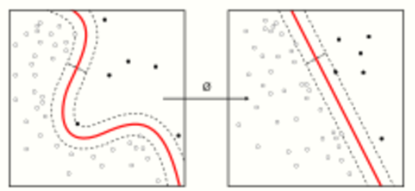
Whereas the original problem may be stated in a finite-dimensional space, it often happens that the sets to discriminate are not linearly separable in that space. For this reason, it was proposed that the original finite-dimensional space be mapped into a much higher-dimensional space, presumably making the separation easier in that space. To keep the computational load reasonable, the mappings used by SVM schemes are designed to ensure that dot products of pairs of input data vectors may be computed easily in terms of the variables in the original space, by defining them in terms of a kernel function [math]\displaystyle{ k(x, y) }[/math] selected to suit the problem.[3] The hyperplanes in the higher-dimensional space are defined as the set of points whose dot product with a vector in that space is constant, where such a set of vectors is an orthogonal (and thus minimal) set of vectors that defines a hyperplane. The vectors defining the hyperplanes can be chosen to be linear combinations with parameters [math]\displaystyle{ \alpha_i }[/math] of images of feature vectors [math]\displaystyle{ x_i }[/math] that occur in the data base.[clarification needed] With this choice of a hyperplane, the points [math]\displaystyle{ x }[/math] in the feature space that are mapped into the hyperplane are defined by the relation [math]\displaystyle{ \textstyle\sum_i \alpha_i k(x_i, x) = \text{constant}. }[/math] Note that if [math]\displaystyle{ k(x, y) }[/math] becomes small as [math]\displaystyle{ y }[/math] grows further away from [math]\displaystyle{ x }[/math], each term in the sum measures the degree of closeness of the test point [math]\displaystyle{ x }[/math] to the corresponding data base point [math]\displaystyle{ x_i }[/math]. In this way, the sum of kernels above can be used to measure the relative nearness of each test point to the data points originating in one or the other of the sets to be discriminated. Note the fact that the set of points [math]\displaystyle{ x }[/math] mapped into any hyperplane can be quite convoluted as a result, allowing much more complex discrimination between sets that are not convex at all in the original space.
3. Applications
SVMs can be used to solve various real-world problems:
- SVMs are helpful in text and hypertext categorization, as their application can significantly reduce the need for labeled training instances in both the standard inductive and transductive settings.[4] Some methods for shallow semantic parsing are based on support vector machines.[5]
- Classification of images can also be performed using SVMs. Experimental results show that SVMs achieve significantly higher search accuracy than traditional query refinement schemes after just three to four rounds of relevance feedback. This is also true for image segmentation systems, including those using a modified version SVM that uses the privileged approach as suggested by Vapnik.[6][7]
- Classification of satellite data like SAR data using supervised SVM.[8]
- Hand-written characters can be recognized using SVM.[9]
- The SVM algorithm has been widely applied in the biological and other sciences. They have been used to classify proteins with up to 90% of the compounds classified correctly. Permutation tests based on SVM weights have been suggested as a mechanism for interpretation of SVM models.[10][11] Support-vector machine weights have also been used to interpret SVM models in the past.[12] Posthoc interpretation of support-vector machine models in order to identify features used by the model to make predictions is a relatively new area of research with special significance in the biological sciences.
4. History
The original SVM algorithm was invented by Vladimir N. Vapnik and Alexey Ya. Chervonenkis in 1963. In 1992, Bernhard Boser, Isabelle Guyon and Vladimir Vapnik suggested a way to create nonlinear classifiers by applying the kernel trick to maximum-margin hyperplanes.[13] The current standard[according to whom?] incarnation (soft margin) was proposed by Corinna Cortes and Vapnik in 1993 and published in 1995.[14]
5. Linear SVM

We are given a training dataset of [math]\displaystyle{ n }[/math] points of the form
- [math]\displaystyle{ (\vec{x}_1, y_1), \ldots, (\vec{x}_n, y_n), }[/math]
where the [math]\displaystyle{ y_i }[/math] are either 1 or −1, each indicating the class to which the point [math]\displaystyle{ \vec{x}_i }[/math] belongs. Each [math]\displaystyle{ \vec{x}_i }[/math] is a [math]\displaystyle{ p }[/math]-dimensional real vector. We want to find the "maximum-margin hyperplane" that divides the group of points [math]\displaystyle{ \vec{x}_i }[/math] for which [math]\displaystyle{ y_i = 1 }[/math] from the group of points for which [math]\displaystyle{ y_i = -1 }[/math], which is defined so that the distance between the hyperplane and the nearest point [math]\displaystyle{ \vec{x}_i }[/math] from either group is maximized.
Any hyperplane can be written as the set of points [math]\displaystyle{ \vec{x} }[/math] satisfying
- [math]\displaystyle{ \vec{w} \cdot \vec{x} - b = 0, }[/math]
where [math]\displaystyle{ \vec{w} }[/math] is the (not necessarily normalized) normal vector to the hyperplane. This is much like Hesse normal form, except that [math]\displaystyle{ \vec{w} }[/math] is not necessarily a unit vector. The parameter [math]\displaystyle{ \tfrac{b}{\|\vec{w}\|} }[/math] determines the offset of the hyperplane from the origin along the normal vector [math]\displaystyle{ \vec{w} }[/math].
5.1. Hard-Margin
If the training data is linearly separable, we can select two parallel hyperplanes that separate the two classes of data, so that the distance between them is as large as possible. The region bounded by these two hyperplanes is called the "margin", and the maximum-margin hyperplane is the hyperplane that lies halfway between them. With a normalized or standardized dataset, these hyperplanes can be described by the equations
- [math]\displaystyle{ \vec{w} \cdot \vec{x} - b = 1 }[/math] (anything on or above this boundary is of one class, with label 1)
and
- [math]\displaystyle{ \vec{w} \cdot \vec{x} - b = -1 }[/math] (anything on or below this boundary is of the other class, with label −1).
Geometrically, the distance between these two hyperplanes is [math]\displaystyle{ \tfrac{2}{\|\vec{w}\|} }[/math],[15] so to maximize the distance between the planes we want to minimize [math]\displaystyle{ \|\vec{w}\| }[/math]. The distance is computed using the distance from a point to a plane equation. We also have to prevent data points from falling into the margin, we add the following constraint: for each [math]\displaystyle{ i }[/math] either
- [math]\displaystyle{ \vec{w} \cdot \vec{x}_i - b \ge 1 }[/math], if [math]\displaystyle{ y_i = 1 }[/math],
or
- [math]\displaystyle{ \vec{w} \cdot \vec{x}_i - b \le -1 }[/math], if [math]\displaystyle{ y_i = -1 }[/math].
These constraints state that each data point must lie on the correct side of the margin.
This can be rewritten as
- [math]\displaystyle{ y_i(\vec{w} \cdot \vec{x}_i - b) \ge 1, \quad \text{ for all } 1 \le i \le n.\qquad\qquad(1) }[/math]
We can put this together to get the optimization problem:
- "Minimize [math]\displaystyle{ \|\vec{w}\| }[/math] subject to [math]\displaystyle{ y_i(\vec{w} \cdot \vec{x}_i - b) \ge 1 }[/math] for [math]\displaystyle{ i = 1, \ldots, n }[/math]."
The [math]\displaystyle{ \vec w }[/math] and [math]\displaystyle{ b }[/math] that solve this problem determine our classifier, [math]\displaystyle{ \vec{x} \mapsto \sgn(\vec{w} \cdot \vec{x} - b) }[/math].
An important consequence of this geometric description is that the max-margin hyperplane is completely determined by those [math]\displaystyle{ \vec{x}_i }[/math] that lie nearest to it. These [math]\displaystyle{ \vec{x}_i }[/math] are called support vectors.
5.2. Soft-Margin
To extend SVM to cases in which the data are not linearly separable, we introduce the hinge loss function,
- [math]\displaystyle{ \max\left(0, 1 - y_i(\vec{w} \cdot \vec{x}_i - b)\right). }[/math]
Note that [math]\displaystyle{ y_i }[/math] is the i-th target (i.e., in this case, 1 or −1), and [math]\displaystyle{ \vec{w} \cdot \vec{x}_i - b }[/math] is the i-th output.
This function is zero if the constraint in (1) is satisfied, in other words, if [math]\displaystyle{ \vec{x}_i }[/math] lies on the correct side of the margin. For data on the wrong side of the margin, the function's value is proportional to the distance from the margin.
We then wish to minimize
- [math]\displaystyle{ \left[\frac 1 n \sum_{i=1}^n \max\left(0, 1 - y_i(\vec{w} \cdot \vec{x}_i - b)\right) \right] + \lambda\lVert \vec{w} \rVert^2, }[/math]
where the parameter [math]\displaystyle{ \lambda }[/math] determines the trade-off between increasing the margin size and ensuring that the [math]\displaystyle{ \vec{x}_i }[/math] lie on the correct side of the margin. Thus, for sufficiently small values of [math]\displaystyle{ \lambda }[/math], the second term in the loss function will become negligible, hence, it will behave similar to the hard-margin SVM, if the input data are linearly classifiable, but will still learn if a classification rule is viable or not.
6. Nonlinear Classification
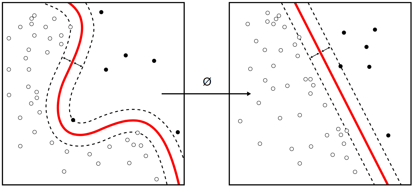
The original maximum-margin hyperplane algorithm proposed by Vapnik in 1963 constructed a linear classifier. However, in 1992, Bernhard Boser, Isabelle Guyon and Vladimir Vapnik suggested a way to create nonlinear classifiers by applying the kernel trick (originally proposed by Aizerman et al.[16]) to maximum-margin hyperplanes.[13] The resulting algorithm is formally similar, except that every dot product is replaced by a nonlinear kernel function. This allows the algorithm to fit the maximum-margin hyperplane in a transformed feature space. The transformation may be nonlinear and the transformed space high-dimensional; although the classifier is a hyperplane in the transformed feature space, it may be nonlinear in the original input space.
It is noteworthy that working in a higher-dimensional feature space increases the generalization error of support-vector machines, although given enough samples the algorithm still performs well.[17]
Some common kernels include:
- Polynomial (homogeneous): [math]\displaystyle{ k(\vec{x_i}, \vec{x_j}) = (\vec{x_i} \cdot \vec{x_j})^d }[/math].
- Polynomial (inhomogeneous): [math]\displaystyle{ k(\vec{x_i}, \vec{x_j}) = (\vec{x_i} \cdot \vec{x_j} + 1)^d }[/math].
- Gaussian radial basis function: [math]\displaystyle{ k(\vec{x_i}, \vec{x_j}) = \exp(-\gamma \|\vec{x_i} - \vec{x_j}\|^2) }[/math] for [math]\displaystyle{ \gamma \gt 0 }[/math]. Sometimes parametrized using [math]\displaystyle{ \gamma = 1/(2\sigma^2) }[/math].
- Hyperbolic tangent: [math]\displaystyle{ k(\vec{x_i}, \vec{x_j}) = \tanh(\kappa \vec{x_i} \cdot \vec{x_j} + c) }[/math] for some (not every) [math]\displaystyle{ \kappa \gt 0 }[/math] and [math]\displaystyle{ c \lt 0 }[/math].
The kernel is related to the transform [math]\displaystyle{ \varphi(\vec{x_i}) }[/math] by the equation [math]\displaystyle{ k(\vec{x_i}, \vec{x_j}) = \varphi(\vec{x_i})\cdot \varphi(\vec{x_j}) }[/math]. The value w is also in the transformed space, with [math]\displaystyle{ \textstyle\vec{w} = \sum_i \alpha_i y_i \varphi(\vec{x}_i) }[/math]. Dot products with w for classification can again be computed by the kernel trick, i.e. [math]\displaystyle{ \textstyle \vec{w} \cdot \varphi(\vec{x}) = \sum_i \alpha_i y_i k(\vec{x}_i, \vec{x}) }[/math].
7. Computing the SVM Classifier
Computing the (soft-margin) SVM classifier amounts to minimizing an expression of the form
- [math]\displaystyle{ \left[\frac 1 n \sum_{i=1}^n \max\left(0, 1 - y_i(w\cdot x_i - b)\right) \right] + \lambda\lVert w \rVert^2. \qquad(2) }[/math]
We focus on the soft-margin classifier since, as noted above, choosing a sufficiently small value for [math]\displaystyle{ \lambda }[/math] yields the hard-margin classifier for linearly classifiable input data. The classical approach, which involves reducing (2) to a quadratic programming problem, is detailed below. Then, more recent approaches such as sub-gradient descent and coordinate descent will be discussed.
7.1. Primal
Minimizing (2) can be rewritten as a constrained optimization problem with a differentiable objective function in the following way.
For each [math]\displaystyle{ i \in \{1,\,\ldots,\,n\} }[/math] we introduce a variable [math]\displaystyle{ \zeta_i = \max\left(0, 1 - y_i(w\cdot x_i - b)\right) }[/math]. Note that [math]\displaystyle{ \zeta_i }[/math] is the smallest nonnegative number satisfying [math]\displaystyle{ y_i(w\cdot x_i - b) \geq 1- \zeta_i. }[/math]
Thus we can rewrite the optimization problem as follows
- [math]\displaystyle{ \text{minimize } \frac 1 n \sum_{i=1}^n \zeta_i + \lambda\|w\|^2 }[/math]
- [math]\displaystyle{ \text{subject to } y_i(w \cdot x_i - b) \geq 1 - \zeta_i \,\text{ and }\,\zeta_i \geq 0,\,\text{for all }i. }[/math]
This is called the primal problem.
7.2. Dual
By solving for the Lagrangian dual of the above problem, one obtains the simplified problem
- [math]\displaystyle{ \text{maximize}\,\, f(c_1 \ldots c_n) = \sum_{i=1}^n c_i - \frac 1 2 \sum_{i=1}^n\sum_{j=1}^n y_ic_i(x_i \cdot x_j)y_jc_j, }[/math]
- [math]\displaystyle{ \text{subject to } \sum_{i=1}^n c_iy_i = 0,\,\text{and } 0 \leq c_i \leq \frac{1}{2n\lambda}\;\text{for all }i. }[/math]
This is called the dual problem. Since the dual maximization problem is a quadratic function of the [math]\displaystyle{ c_i }[/math] subject to linear constraints, it is efficiently solvable by quadratic programming algorithms.
Here, the variables [math]\displaystyle{ c_i }[/math] are defined such that
- [math]\displaystyle{ \vec w = \sum_{i=1}^n c_iy_i \vec x_i }[/math].
Moreover, [math]\displaystyle{ c_i = 0 }[/math] exactly when [math]\displaystyle{ \vec x_i }[/math] lies on the correct side of the margin, and [math]\displaystyle{ 0 \lt c_i \lt (2n\lambda)^{-1} }[/math] when [math]\displaystyle{ \vec x_i }[/math] lies on the margin's boundary. It follows that [math]\displaystyle{ \vec w }[/math] can be written as a linear combination of the support vectors.
The offset, [math]\displaystyle{ b }[/math], can be recovered by finding an [math]\displaystyle{ \vec x_i }[/math] on the margin's boundary and solving
- [math]\displaystyle{ y_i(\vec w \cdot \vec x_i - b) = 1 \iff b = \vec w \cdot \vec x_i - y_i . }[/math]
(Note that [math]\displaystyle{ y_i^{-1}=y_i }[/math] since [math]\displaystyle{ y_i=\pm 1 }[/math].)
7.3. Kernel Trick
Suppose now that we would like to learn a nonlinear classification rule which corresponds to a linear classification rule for the transformed data points [math]\displaystyle{ \varphi(\vec x_i). }[/math] Moreover, we are given a kernel function [math]\displaystyle{ k }[/math] which satisfies [math]\displaystyle{ k(\vec x_i, \vec x_j) = \varphi(\vec x_i) \cdot \varphi(\vec x_j) }[/math].
We know the classification vector [math]\displaystyle{ \vec w }[/math] in the transformed space satisfies
- [math]\displaystyle{ \vec w = \sum_{i=1}^n c_iy_i\varphi( \vec x_i), }[/math]
where, the [math]\displaystyle{ c_i }[/math] are obtained by solving the optimization problem
- [math]\displaystyle{ \begin{align} \text{maximize}\,\, f(c_1 \ldots c_n) &= \sum_{i=1}^n c_i - \frac 1 2 \sum_{i=1}^n\sum_{j=1}^n y_ic_i(\varphi(\vec x_i) \cdot \varphi(\vec x_j))y_jc_j \\ &= \sum_{i=1}^n c_i - \frac 1 2 \sum_{i=1}^n\sum_{j=1}^n y_ic_ik(\vec x_i,\vec x_j)y_jc_j \\ \end{align} }[/math]
- [math]\displaystyle{ \text{subject to } \sum_{i=1}^n c_iy_i = 0,\,\text{and } 0 \leq c_i \leq \frac{1}{2n\lambda}\;\text{for all }i. }[/math]
The coefficients [math]\displaystyle{ c_i }[/math] can be solved for using quadratic programming, as before. Again, we can find some index [math]\displaystyle{ i }[/math] such that [math]\displaystyle{ 0 \lt c_i \lt (2n\lambda)^{-1} }[/math], so that [math]\displaystyle{ \varphi(\vec x_i) }[/math] lies on the boundary of the margin in the transformed space, and then solve
- [math]\displaystyle{ \begin{align} b = \vec w \cdot \varphi(\vec x_i) - y_i &= \left[\sum_{j=1}^n c_jy_j\varphi(\vec x_j)\cdot\varphi(\vec x_i)\right] - y_i \\ &= \left[\sum_{j=1}^n c_jy_jk(\vec x_j, \vec x_i)\right] - y_i. \end{align} }[/math]
Finally,
- [math]\displaystyle{ \vec z \mapsto \sgn(\vec w \cdot \varphi(\vec z) - b) = \sgn\left(\left[\sum_{i=1}^n c_iy_ik(\vec x_i, \vec z)\right] - b\right). }[/math]
7.4. Modern Methods
Recent algorithms for finding the SVM classifier include sub-gradient descent and coordinate descent. Both techniques have proven to offer significant advantages over the traditional approach when dealing with large, sparse datasets—sub-gradient methods are especially efficient when there are many training examples, and coordinate descent when the dimension of the feature space is high.
Sub-gradient descent
Sub-gradient descent algorithms for the SVM work directly with the expression
- [math]\displaystyle{ f(\vec w, b) = \left[\frac 1 n \sum_{i=1}^n \max\left(0, 1 - y_i(\vec w\cdot \vec x_i - b)\right) \right] + \lambda\lVert \vec w \rVert^2. }[/math]
Note that [math]\displaystyle{ f }[/math] is a convex function of [math]\displaystyle{ \vec w }[/math] and [math]\displaystyle{ b }[/math]. As such, traditional gradient descent (or SGD) methods can be adapted, where instead of taking a step in the direction of the function's gradient, a step is taken in the direction of a vector selected from the function's sub-gradient. This approach has the advantage that, for certain implementations, the number of iterations does not scale with [math]\displaystyle{ n }[/math], the number of data points.[18]
Coordinate descent
Coordinate descent algorithms for the SVM work from the dual problem
- [math]\displaystyle{ \text{maximize}\,\, f(c_1 \ldots c_n) = \sum_{i=1}^n c_i - \frac 1 2 \sum_{i=1}^n\sum_{j=1}^n y_ic_i(x_i \cdot x_j)y_jc_j, }[/math]
- [math]\displaystyle{ \text{subject to } \sum_{i=1}^n c_iy_i = 0,\,\text{and } 0 \leq c_i \leq \frac{1}{2n\lambda}\;\text{for all }i. }[/math]
For each [math]\displaystyle{ i \in \{1,\, \ldots,\, n\} }[/math], iteratively, the coefficient [math]\displaystyle{ c_i }[/math] is adjusted in the direction of [math]\displaystyle{ \partial f/ \partial c_i }[/math]. Then, the resulting vector of coefficients [math]\displaystyle{ (c_1',\,\ldots,\,c_n') }[/math] is projected onto the nearest vector of coefficients that satisfies the given constraints. (Typically Euclidean distances are used.) The process is then repeated until a near-optimal vector of coefficients is obtained. The resulting algorithm is extremely fast in practice, although few performance guarantees have been proven.[19]
8. Empirical Risk Minimization
The soft-margin support vector machine described above is an example of an empirical risk minimization (ERM) algorithm for the hinge loss. Seen this way, support vector machines belong to a natural class of algorithms for statistical inference, and many of its unique features are due to the behavior of the hinge loss. This perspective can provide further insight into how and why SVMs work, and allow us to better analyze their statistical properties.
8.1. Risk Minimization
In supervised learning, one is given a set of training examples [math]\displaystyle{ X_1 \ldots X_n }[/math] with labels [math]\displaystyle{ y_1 \ldots y_n }[/math], and wishes to predict [math]\displaystyle{ y_{n+1} }[/math] given [math]\displaystyle{ X_{n+1} }[/math]. To do so one forms a hypothesis, [math]\displaystyle{ f }[/math], such that [math]\displaystyle{ f(X_{n+1}) }[/math] is a "good" approximation of [math]\displaystyle{ y_{n+1} }[/math]. A "good" approximation is usually defined with the help of a loss function, [math]\displaystyle{ \ell(y,z) }[/math], which characterizes how bad [math]\displaystyle{ z }[/math] is as a prediction of [math]\displaystyle{ y }[/math]. We would then like to choose a hypothesis that minimizes the expected risk:
- [math]\displaystyle{ \varepsilon(f) = \mathbb{E}\left[\ell(y_{n+1}, f(X_{n+1})) \right]. }[/math]
In most cases, we don't know the joint distribution of [math]\displaystyle{ X_{n+1},\,y_{n+1} }[/math] outright. In these cases, a common strategy is to choose the hypothesis that minimizes the empirical risk:
- [math]\displaystyle{ \hat \varepsilon(f) = \frac 1 n \sum_{k=1}^n \ell(y_k, f(X_k)). }[/math]
Under certain assumptions about the sequence of random variables [math]\displaystyle{ X_k,\, y_k }[/math] (for example, that they are generated by a finite Markov process), if the set of hypotheses being considered is small enough, the minimizer of the empirical risk will closely approximate the minimizer of the expected risk as [math]\displaystyle{ n }[/math] grows large. This approach is called empirical risk minimization, or ERM.
8.2. Regularization and Stability
In order for the minimization problem to have a well-defined solution, we have to place constraints on the set [math]\displaystyle{ \mathcal{H} }[/math] of hypotheses being considered. If [math]\displaystyle{ \mathcal{H} }[/math] is a normed space (as is the case for SVM), a particularly effective technique is to consider only those hypotheses [math]\displaystyle{ f }[/math] for which [math]\displaystyle{ \lVert f \rVert_{\mathcal H} \lt k }[/math] . This is equivalent to imposing a regularization penalty [math]\displaystyle{ \mathcal R(f) = \lambda_k\lVert f \rVert_{\mathcal H} }[/math], and solving the new optimization problem
- [math]\displaystyle{ \hat f = \mathrm{arg}\min_{f \in \mathcal{H}} \hat \varepsilon(f) + \mathcal{R}(f). }[/math]
This approach is called Tikhonov regularization.
More generally, [math]\displaystyle{ \mathcal{R}(f) }[/math] can be some measure of the complexity of the hypothesis [math]\displaystyle{ f }[/math], so that simpler hypotheses are preferred.
8.3. SVM and the Hinge Loss
Recall that the (soft-margin) SVM classifier [math]\displaystyle{ \hat w, b: x \mapsto \sgn(\hat w \cdot x - b) }[/math] is chosen to minimize the following expression:
- [math]\displaystyle{ \left[\frac 1 n \sum_{i=1}^n \max\left(0, 1 - y_i(w\cdot x_i - b)\right) \right] + \lambda\lVert w \rVert^2. }[/math]
In light of the above discussion, we see that the SVM technique is equivalent to empirical risk minimization with Tikhonov regularization, where in this case the loss function is the hinge loss
- [math]\displaystyle{ \ell(y,z) = \max\left(0, 1 - yz \right). }[/math]
From this perspective, SVM is closely related to other fundamental classification algorithms such as regularized least-squares and logistic regression. The difference between the three lies in the choice of loss function: regularized least-squares amounts to empirical risk minimization with the square-loss, [math]\displaystyle{ \ell_{sq}(y,z) = (y-z)^2 }[/math]; logistic regression employs the log-loss,
- [math]\displaystyle{ \ell_{\log}(y,z) = \ln(1 + e^{-yz}). }[/math]
Target functions
The difference between the hinge loss and these other loss functions is best stated in terms of target functions - the function that minimizes expected risk for a given pair of random variables [math]\displaystyle{ X,\,y }[/math].
In particular, let [math]\displaystyle{ y_x }[/math] denote [math]\displaystyle{ y }[/math] conditional on the event that [math]\displaystyle{ X = x }[/math]. In the classification setting, we have:
- [math]\displaystyle{ y_x = \begin{cases} 1 & \text{with probability } p_x \\ -1 & \text{with probability } 1-p_x \end{cases} }[/math]
The optimal classifier is therefore:
- [math]\displaystyle{ f^*(x) = \begin{cases}1 & \text{if }p_x \geq 1/2 \\ -1 & \text{otherwise}\end{cases} }[/math]
For the square-loss, the target function is the conditional expectation function, [math]\displaystyle{ f_{sq}(x) = \mathbb{E}\left[y_x\right] }[/math]; For the logistic loss, it's the logit function, [math]\displaystyle{ f_{\log}(x) = \ln\left(p_x / ({1-p_x})\right) }[/math]. While both of these target functions yield the correct classifier, they give us more information than we need. In fact, they give us enough information to completely describe the distribution of [math]\displaystyle{ y_x }[/math].
On the other hand, one can check that the target function for the hinge loss is exactly [math]\displaystyle{ f^* }[/math]. Thus, in a sufficiently rich hypothesis space—or equivalently, for an appropriately chosen kernel—the SVM classifier will converge to the simplest function (in terms of [math]\displaystyle{ \mathcal{R} }[/math]) that correctly classifies the data. This extends the geometric interpretation of SVM—for linear classification, the empirical risk is minimized by any function whose margins lie between the support vectors, and the simplest of these is the max-margin classifier.[20]
9. Properties
SVMs belong to a family of generalized linear classifiers and can be interpreted as an extension of the perceptron. They can also be considered a special case of Tikhonov regularization. A special property is that they simultaneously minimize the empirical classification error and maximize the geometric margin; hence they are also known as maximum margin classifiers.
A comparison of the SVM to other classifiers has been made by Meyer, Leisch and Hornik.[21]
9.1. Parameter Selection
The effectiveness of SVM depends on the selection of kernel, the kernel's parameters, and soft margin parameter C. A common choice is a Gaussian kernel, which has a single parameter [math]\displaystyle{ \gamma }[/math]. The best combination of C and [math]\displaystyle{ \gamma }[/math] is often selected by a grid search with exponentially growing sequences of C and [math]\displaystyle{ \gamma }[/math], for example, [math]\displaystyle{ C \in \{ 2^{-5}, 2^{-3}, \dots, 2^{13},2^{15} \} }[/math]; [math]\displaystyle{ \gamma \in \{ 2^{-15},2^{-13}, \dots, 2^{1},2^{3} \} }[/math]. Typically, each combination of parameter choices is checked using cross validation, and the parameters with best cross-validation accuracy are picked. Alternatively, recent work in Bayesian optimization can be used to select C and [math]\displaystyle{ \gamma }[/math] , often requiring the evaluation of far fewer parameter combinations than grid search. The final model, which is used for testing and for classifying new data, is then trained on the whole training set using the selected parameters.[22]
9.2. Issues
Potential drawbacks of the SVM include the following aspects:
- Requires full labeling of input data
- Uncalibrated class membership probabilities—SVM stems from Vapnik's theory which avoids estimating probabilities on finite data
- The SVM is only directly applicable for two-class tasks. Therefore, algorithms that reduce the multi-class task to several binary problems have to be applied; see the multi-class SVM section.
- Parameters of a solved model are difficult to interpret.
10. Extensions
10.1. Support-Vector Clustering (SVC)
SVC is a similar method that also builds on kernel functions but is appropriate for unsupervised learning. It is considered a fundamental method in data science.
10.2. Multiclass SVM
Multiclass SVM aims to assign labels to instances by using support-vector machines, where the labels are drawn from a finite set of several elements.
The dominant approach for doing so is to reduce the single multiclass problem into multiple binary classification problems.[23] Common methods for such reduction include:[23][24]
- Building binary classifiers that distinguish between one of the labels and the rest (one-versus-all) or between every pair of classes (one-versus-one). Classification of new instances for the one-versus-all case is done by a winner-takes-all strategy, in which the classifier with the highest-output function assigns the class (it is important that the output functions be calibrated to produce comparable scores). For the one-versus-one approach, classification is done by a max-wins voting strategy, in which every classifier assigns the instance to one of the two classes, then the vote for the assigned class is increased by one vote, and finally the class with the most votes determines the instance classification.
- Directed acyclic graph SVM (DAGSVM)[25]
- Error-correcting output codes[26]
Crammer and Singer proposed a multiclass SVM method which casts the multiclass classification problem into a single optimization problem, rather than decomposing it into multiple binary classification problems.[27] See also Lee, Lin and Wahba[28][29] and Van den Burg and Groenen.[30]
10.3. Transductive Support-Vector Machines
Transductive support-vector machines extend SVMs in that they could also treat partially labeled data in semi-supervised learning by following the principles of transduction. Here, in addition to the training set [math]\displaystyle{ \mathcal{D} }[/math], the learner is also given a set
- [math]\displaystyle{ \mathcal{D}^\star = \{ \vec{x}^\star_i \mid \vec{x}^\star_i \in \mathbb{R}^p\}_{i=1}^k }[/math]
of test examples to be classified. Formally, a transductive support-vector machine is defined by the following primal optimization problem:[31]
Minimize (in [math]\displaystyle{ {\vec{w}, b, \vec{y^\star}} }[/math])
- [math]\displaystyle{ \frac{1}{2}\|\vec{w}\|^2 }[/math]
subject to (for any [math]\displaystyle{ i = 1, \dots, n }[/math] and any [math]\displaystyle{ j = 1, \dots, k }[/math])
- [math]\displaystyle{ y_i(\vec{w} \cdot \vec{x_i} - b) \ge 1, }[/math]
- [math]\displaystyle{ y^\star_j(\vec{w} \cdot \vec{x^\star_j} - b) \ge 1, }[/math]
and
- [math]\displaystyle{ y^\star_j \in \{-1, 1\}. }[/math]
Transductive support-vector machines were introduced by Vladimir N. Vapnik in 1998.
10.4. Structured SVM
SVMs have been generalized to structured SVMs, where the label space is structured and of possibly infinite size.
10.5. Regression
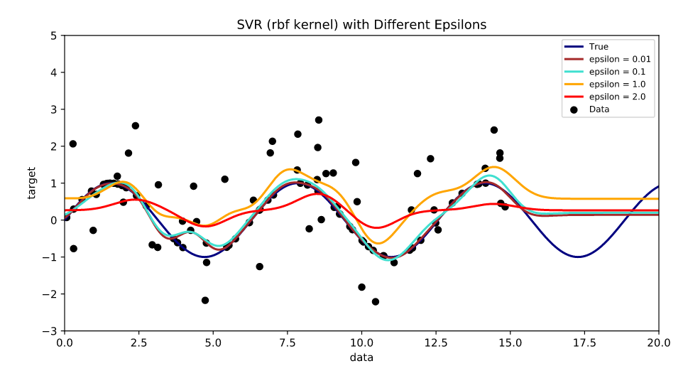
A version of SVM for regression was proposed in 1996 by Vladimir N. Vapnik, Harris Drucker, Christopher J. C. Burges, Linda Kaufman and Alexander J. Smola.[32] This method is called support-vector regression (SVR). The model produced by support-vector classification (as described above) depends only on a subset of the training data, because the cost function for building the model does not care about training points that lie beyond the margin. Analogously, the model produced by SVR depends only on a subset of the training data, because the cost function for building the model ignores any training data close to the model prediction. Another SVM version known as least-squares support-vector machine (LS-SVM) has been proposed by Suykens and Vandewalle.[33]
Training the original SVR means solving[34]
- minimize [math]\displaystyle{ \frac{1}{2} \|w\|^2 }[/math]
- subject to [math]\displaystyle{ | y_i - \langle w, x_i \rangle - b | \le \varepsilon }[/math]
where [math]\displaystyle{ x_i }[/math] is a training sample with target value [math]\displaystyle{ y_i }[/math]. The inner product plus intercept [math]\displaystyle{ \langle w, x_i \rangle + b }[/math] is the prediction for that sample, and [math]\displaystyle{ \varepsilon }[/math] is a free parameter that serves as a threshold: all predictions have to be within an [math]\displaystyle{ \varepsilon }[/math] range of the true predictions. Slack variables are usually added into the above to allow for errors and to allow approximation in the case the above problem is infeasible.
10.6. Bayesian SVM
In 2011 it was shown by Polson and Scott that the SVM admits a Bayesian interpretation through the technique of data augmentation.[35] In this approach the SVM is viewed as a graphical model (where the parameters are connected via probability distributions). This extended view allows the application of Bayesian techniques to SVMs, such as flexible feature modeling, automatic hyperparameter tuning, and predictive uncertainty quantification. Recently, a scalable version of the Bayesian SVM was developed by Florian Wenzel, enabling the application of Bayesian SVMs to big data.[36] Florian Wenzel developed two different versions, a variational inference (VI) scheme for the Bayesian kernel support vector machine (SVM) and a stochastic version (SVI) for the linear Bayesian SVM.[37]
11. Implementation
The parameters of the maximum-margin hyperplane are derived by solving the optimization. There exist several specialized algorithms for quickly solving the quadratic programming (QP) problem that arises from SVMs, mostly relying on heuristics for breaking the problem down into smaller, more manageable chunks.
Another approach is to use an interior-point method that uses Newton-like iterations to find a solution of the Karush–Kuhn–Tucker conditions of the primal and dual problems.[38] Instead of solving a sequence of broken-down problems, this approach directly solves the problem altogether. To avoid solving a linear system involving the large kernel matrix, a low-rank approximation to the matrix is often used in the kernel trick.
Another common method is Platt's sequential minimal optimization (SMO) algorithm, which breaks the problem down into 2-dimensional sub-problems that are solved analytically, eliminating the need for a numerical optimization algorithm and matrix storage. This algorithm is conceptually simple, easy to implement, generally faster, and has better scaling properties for difficult SVM problems.[39]
The special case of linear support-vector machines can be solved more efficiently by the same kind of algorithms used to optimize its close cousin, logistic regression; this class of algorithms includes sub-gradient descent (e.g., PEGASOS[40]) and coordinate descent (e.g., LIBLINEAR[41]). LIBLINEAR has some attractive training-time properties. Each convergence iteration takes time linear in the time taken to read the train data, and the iterations also have a Q-linear convergence property, making the algorithm extremely fast.
The general kernel SVMs can also be solved more efficiently using sub-gradient descent (e.g. P-packSVM[42]), especially when parallelization is allowed.
Kernel SVMs are available in many machine-learning toolkits, including LIBSVM, MATLAB, SAS, SVMlight, kernlab, scikit-learn, Shogun, Weka, Shark, JKernelMachines, OpenCV and others.
References
- "1.4. Support Vector Machines — scikit-learn 0.20.2 documentation". http://scikit-learn.org/stable/modules/svm.html.
- Hastie, Trevor; Tibshirani, Robert; Friedman, Jerome (2008). The Elements of Statistical Learning : Data Mining, Inference, and Prediction (Second ed.). New York: Springer. p. 134. https://web.stanford.edu/~hastie/Papers/ESLII.pdf#page=153.
- Press, William H.; Teukolsky, Saul A.; Vetterling, William T.; Flannery, Brian P. (2007). "Section 16.5. Support Vector Machines". Numerical Recipes: The Art of Scientific Computing (3rd ed.). New York: Cambridge University Press. ISBN 978-0-521-88068-8. http://apps.nrbook.com/empanel/index.html#pg=883.
- Joachims, Thorsten (1998). "Text categorization with Support Vector Machines: Learning with many relevant features" (in en). Machine Learning: ECML-98. Lecture Notes in Computer Science (Springer) 1398: 137–142. doi:10.1007/BFb0026683. ISBN 978-3-540-64417-0. https://dx.doi.org/10.1007%2FBFb0026683
- Pradhan, Sameer S., et al. "Shallow semantic parsing using support vector machines." Proceedings of the Human Language Technology Conference of the North American Chapter of the Association for Computational Linguistics: HLT-NAACL 2004. 2004. http://www.aclweb.org/anthology/N04-1030
- Vapnik, Vladimir N.: Invited Speaker. IPMU Information Processing and Management 2014).
- Barghout, Lauren. "Spatial-Taxon Information Granules as Used in Iterative Fuzzy-Decision-Making for Image Segmentation". Granular Computing and Decision-Making. Springer International Publishing, 2015. 285–318. https://pdfs.semanticscholar.org/917f/15d33d32062bffeb6401eee9fe71d16d6a84.pdf
- A. Maity (2016). "Supervised Classification of RADARSAT-2 Polarimetric Data for Different Land Features". arXiv:1608.00501 [cs.CV]. //arxiv.org/archive/cs.CV
- DeCoste, Dennis (2002). "Training Invariant Support Vector Machines". Machine Learning 46: 161–190. doi:10.1023/A:1012454411458. https://people.eecs.berkeley.edu/~malik/cs294/decoste-scholkopf.pdf.
- Gaonkar, Bilwaj; Davatzikos, Christos; "Analytic estimation of statistical significance maps for support vector machine based multi-variate image analysis and classification". https://www.ncbi.nlm.nih.gov/pmc/articles/PMC3767485/
- Cuingnet, Rémi; Rosso, Charlotte; Chupin, Marie; Lehéricy, Stéphane; Dormont, Didier; Benali, Habib; Samson, Yves; and Colliot, Olivier; "Spatial regularization of SVM for the detection of diffusion alterations associated with stroke outcome", Medical Image Analysis, 2011, 15 (5): 729–737. http://www.aramislab.fr/perso/colliot/files/media2011_remi_published.pdf
- Statnikov, Alexander; Hardin, Douglas; & Aliferis, Constantin; (2006); "Using SVM weight-based methods to identify causally relevant and non-causally relevant variables", Sign, 1, 4. http://www.ccdlab.org/paper-pdfs/NIPS_2006.pdf
- Boser, Bernhard E.; Guyon, Isabelle M.; Vapnik, Vladimir N. (1992). "A training algorithm for optimal margin classifiers". Proceedings of the fifth annual workshop on Computational learning theory – COLT '92. pp. 144. doi:10.1145/130385.130401. ISBN 978-0897914970. http://www.clopinet.com/isabelle/Papers/colt92.ps.Z.
- Cortes, Corinna; Vapnik, Vladimir N. (1995). "Support-vector networks". Machine Learning 20 (3): 273–297. doi:10.1007/BF00994018. http://image.diku.dk/imagecanon/material/cortes_vapnik95.pdf.
- "Why does the SVM margin is [math]\displaystyle{ \frac{\|\mathbf\|} }[/math]". 30 May 2015. https://math.stackexchange.com/q/1305925/168764.
- Aizerman, Mark A.; Braverman, Emmanuel M.; Rozonoer, Lev I. (1964). "Theoretical foundations of the potential function method in pattern recognition learning". Automation and Remote Control 25: 821–837.
- Jin, Chi; Wang, Liwei (2012). "Dimensionality dependent PAC-Bayes margin bound". Advances in Neural Information Processing Systems. http://papers.nips.cc/paper/4500-dimensionality-dependent-pac-bayes-margin-bound.
- Shalev-Shwartz, Shai; Singer, Yoram; Srebro, Nathan; Cotter, Andrew (2010-10-16). "Pegasos: primal estimated sub-gradient solver for SVM". Mathematical Programming 127 (1): 3–30. doi:10.1007/s10107-010-0420-4. ISSN 0025-5610. https://dx.doi.org/10.1007%2Fs10107-010-0420-4
- Hsieh, Cho-Jui; Chang, Kai-Wei; Lin, Chih-Jen; Keerthi, S. Sathiya; Sundararajan, S. (2008-01-01). A Dual Coordinate Descent Method for Large-scale Linear SVM. ICML '08. New York, NY, USA: ACM. 408–415. doi:10.1145/1390156.1390208. ISBN 978-1-60558-205-4. https://dx.doi.org/10.1145%2F1390156.1390208
- Rosasco, Lorenzo; De Vito, Ernesto; Caponnetto, Andrea; Piana, Michele; Verri, Alessandro (2004-05-01). "Are Loss Functions All the Same?". Neural Computation 16 (5): 1063–1076. doi:10.1162/089976604773135104. ISSN 0899-7667. PMID 15070510. https://ieeexplore.ieee.org/document/6789841.
- Meyer, David; Leisch, Friedrich; Hornik, Kurt (September 2003). "The support vector machine under test". Neurocomputing 55 (1–2): 169–186. doi:10.1016/S0925-2312(03)00431-4. https://dx.doi.org/10.1016%2FS0925-2312%2803%2900431-4
- Hsu, Chih-Wei; Chang, Chih-Chung & Lin, Chih-Jen (2003). A Practical Guide to Support Vector Classification (PDF) (Technical report). Department of Computer Science and Information Engineering, National Taiwan University. Archived (PDF) from the original on 2013-06-25. Cite uses deprecated parameter |last-author-amp= (help) http://www.csie.ntu.edu.tw/~cjlin/papers/guide/guide.pdf
- Duan, Kai-Bo; Keerthi, S. Sathiya (2005). "Which Is the Best Multiclass SVM Method? An Empirical Study". Multiple Classifier Systems. LNCS. 3541. pp. 278–285. doi:10.1007/11494683_28. ISBN 978-3-540-26306-7. https://www.cs.iastate.edu/~honavar/multiclass-svm2.pdf.
- Hsu, Chih-Wei; Lin, Chih-Jen (2002). "A Comparison of Methods for Multiclass Support Vector Machines". IEEE Transactions on Neural Networks 13 (2): 415–25. doi:10.1109/72.991427. PMID 18244442. http://www.cs.iastate.edu/~honavar/multiclass-svm.pdf.
- Platt, John; Cristianini, Nello; Shawe-Taylor, John (2000). "Large margin DAGs for multiclass classification". Advances in Neural Information Processing Systems. MIT Press. pp. 547–553. http://www.wisdom.weizmann.ac.il/~bagon/CVspring07/files/DAGSVM.pdf.
- Dietterich, Thomas G.; Bakiri, Ghulum (1995). "Solving Multiclass Learning Problems via Error-Correcting Output Codes". Journal of Artificial Intelligence Research 2: 263–286. doi:10.1613/jair.105. Bibcode: 1995cs........1101D. http://www.jair.org/media/105/live-105-1426-jair.pdf.
- Crammer, Koby; Singer, Yoram (2001). "On the Algorithmic Implementation of Multiclass Kernel-based Vector Machines". Journal of Machine Learning Research 2: 265–292. http://jmlr.csail.mit.edu/papers/volume2/crammer01a/crammer01a.pdf.
- Lee, Yoonkyung; Lin, Yi; Wahba, Grace (2001). "Multicategory Support Vector Machines". Computing Science and Statistics 33. http://www.interfacesymposia.org/I01/I2001Proceedings/YLee/YLee.pdf.
- Lee, Yoonkyung; Lin, Yi; Wahba, Grace (2004). "Multicategory Support Vector Machines". Journal of the American Statistical Association 99 (465): 67–81. doi:10.1198/016214504000000098. https://dx.doi.org/10.1198%2F016214504000000098
- Van den Burg, Gerrit J. J.; Groenen, Patrick J. F. (2016). "GenSVM: A Generalized Multiclass Support Vector Machine". Journal of Machine Learning Research 17 (224): 1–42. http://jmlr.org/papers/volume17/14-526/14-526.pdf.
- Joachims, Thorsten; "Transductive Inference for Text Classification using Support Vector Machines", Proceedings of the 1999 International Conference on Machine Learning (ICML 1999), pp. 200–209. http://www1.cs.columbia.edu/~dplewis/candidacy/joachims99transductive.pdf
- Drucker, Harris; Burges, Christ. C.; Kaufman, Linda; Smola, Alexander J.; and Vapnik, Vladimir N. (1997); "Support Vector Regression Machines", in Advances in Neural Information Processing Systems 9, NIPS 1996, 155–161, MIT Press. http://papers.nips.cc/paper/1238-support-vector-regression-machines.pdf
- Suykens, Johan A. K.; Vandewalle, Joos P. L.; "Least squares support vector machine classifiers", Neural Processing Letters, vol. 9, no. 3, Jun. 1999, pp. 293–300. https://lirias.kuleuven.be/bitstream/123456789/218716/2/Suykens_NeurProcLett.pdf
- Smola, Alex J.; Schölkopf, Bernhard (2004). "A tutorial on support vector regression". Statistics and Computing 14 (3): 199–222. doi:10.1023/B:STCO.0000035301.49549.88. http://eprints.pascal-network.org/archive/00000856/01/fulltext.pdf.
- Polson, Nicholas G.; Scott, Steven L. (2011). "Data Augmentation for Support Vector Machines". Bayesian Analysis 6 (1): 1–23. doi:10.1214/11-BA601. https://dx.doi.org/10.1214%2F11-BA601
- Wenzel, Florian; Galy-Fajou, Theo; Deutsch, Matthäus; Kloft, Marius (2017). "Bayesian Nonlinear Support Vector Machines for Big Data". Machine Learning and Knowledge Discovery in Databases (ECML PKDD). Lecture Notes in Computer Science 10534: 307–322. doi:10.1007/978-3-319-71249-9_19. ISBN 978-3-319-71248-2. Bibcode: 2017arXiv170705532W. Archived on 2017-08-30. Error: If you specify |archivedate=, you must first specify |url=. https://dx.doi.org/10.1007%2F978-3-319-71249-9_19
- Florian Wenzel; Matthäus Deutsch; Théo Galy-Fajou; Marius Kloft; ”Scalable Approximate Inference for the Bayesian Nonlinear Support Vector Machine” https://amor.cms.hu-berlin.de/~wenzelfl/files/nips_bayesianSVM_2016.pdf
- Ferris, Michael C.; Munson, Todd S. (2002). "Interior-Point Methods for Massive Support Vector Machines". SIAM Journal on Optimization 13 (3): 783–804. doi:10.1137/S1052623400374379. http://www.cs.wisc.edu/~ferris/papers/siopt-svm.pdf.
- Platt, John C. (1998). "Sequential Minimal Optimization: A Fast Algorithm for Training Support Vector Machines". NIPS. http://research.microsoft.com/pubs/69644/tr-98-14.pdf.
- Shalev-Shwartz, Shai; Singer, Yoram; Srebro, Nathan (2007). "Pegasos: Primal Estimated sub-GrAdient SOlver for SVM". ICML. http://ttic.uchicago.edu/~shai/papers/ShalevSiSr07.pdf.
- Fan, Rong-En; Chang, Kai-Wei; Hsieh, Cho-Jui; Wang, Xiang-Rui; Lin, Chih-Jen (2008). "LIBLINEAR: A library for large linear classification". Journal of Machine Learning Research 9: 1871–1874. https://www.csie.ntu.edu.tw/~cjlin/papers/liblinear.pdf.
- Allen Zhu, Zeyuan; Chen, Weizhu; Wang, Gang; Zhu, Chenguang; Chen, Zheng (2009). "P-packSVM: Parallel Primal grAdient desCent Kernel SVM". ICDM. http://people.csail.mit.edu/zeyuan/paper/2009-ICDM-Parallel.pdf.

