 +1 credit
| Version | Summary | Created by | Modification | Content Size | Created at | Operation |
|---|---|---|---|---|---|---|
| 1 | Beatrix Zheng | -- | 3791 | 2022-10-14 01:36:33 |
Video Upload Options
In statistics, correlation or dependence is any statistical relationship, whether causal or not, between two random variables or bivariate data. In the broadest sense correlation is any statistical association, though it commonly refers to the degree to which a pair of variables are linearly related. Familiar examples of dependent phenomena include the correlation between the height of parents and their offspring, and the correlation between the price of a good and the quantity the consumers are willing to purchase, as it is depicted in the so-called demand curve. Correlations are useful because they can indicate a predictive relationship that can be exploited in practice. For example, an electrical utility may produce less power on a mild day based on the correlation between electricity demand and weather. In this example, there is a causal relationship, because extreme weather causes people to use more electricity for heating or cooling. However, in general, the presence of a correlation is not sufficient to infer the presence of a causal relationship (i.e., correlation does not imply causation). Formally, random variables are dependent if they do not satisfy a mathematical property of probabilistic independence. In informal parlance, correlation is synonymous with dependence. However, when used in a technical sense, correlation refers to any of several specific types of mathematical operations between the tested variables and their respective expected values. Essentially, correlation is the measure of how two or more variables are related to one another. There are several correlation coefficients, often denoted [math]\displaystyle{ \rho }[/math] or [math]\displaystyle{ r }[/math], measuring the degree of correlation. The most common of these is the Pearson correlation coefficient, which is sensitive only to a linear relationship between two variables (which may be present even when one variable is a nonlinear function of the other). Other correlation coefficients – such as Spearman's rank correlation – have been developed to be more robust than Pearson's, that is, more sensitive to nonlinear relationships. Mutual information can also be applied to measure dependence between two variables.
1. Pearson's Product-moment Coefficient
1.1. Definition
The most familiar measure of dependence between two quantities is the Pearson product-moment correlation coefficient (PPMCC), or "Pearson's correlation coefficient", commonly called simply "the correlation coefficient". Mathematically, it is defined as the quality of least squares fitting to the original data. It is obtained by taking the ratio of the covariance of the two variables in question of our numerical dataset, normalized to the square root of their variances. Mathematically, one simply divides the covariance of the two variables by the product of their standard deviations. Karl Pearson developed the coefficient from a similar but slightly different idea by Francis Galton.[1]
A Pearson product-moment correlation coefficient attempts to establish a line of best fit through a dataset of two variables by essentially laying out the expected values and the resulting Pearson's correlation coefficient indicates how far away the actual dataset is from the expected values. Depending on the sign of our Pearson's correlation coefficient, we can end up with either a negative or positive correlation if there is any sort of relationship between the variables of our data set.
The population correlation coefficient [math]\displaystyle{ \rho_{X,Y} }[/math] between two random variables [math]\displaystyle{ X }[/math] and [math]\displaystyle{ Y }[/math] with expected values [math]\displaystyle{ \mu_X }[/math] and [math]\displaystyle{ \mu_Y }[/math] and standard deviations [math]\displaystyle{ \sigma_X }[/math] and [math]\displaystyle{ \sigma_Y }[/math] is defined as
[math]\displaystyle{ \rho_{X,Y} = \operatorname{corr}(X,Y) = {\operatorname{cov}(X,Y) \over \sigma_X \sigma_Y} = {\operatorname{E}[(X-\mu_X)(Y-\mu_Y)] \over \sigma_X\sigma_Y} }[/math]
where [math]\displaystyle{ \operatorname{E} }[/math] is the expected value operator, [math]\displaystyle{ \operatorname{cov} }[/math] means covariance, and [math]\displaystyle{ \operatorname{corr} }[/math] is a widely used alternative notation for the correlation coefficient. The Pearson correlation is defined only if both standard deviations are finite and positive. An alternative formula purely in terms of moments is
[math]\displaystyle{ \rho_{X,Y} = {\operatorname{E}(XY)-\operatorname{E}(X)\operatorname{E}(Y)\over \sqrt{\operatorname{E}(X^2)-\operatorname{E}(X)^2}\cdot \sqrt{\operatorname{E}(Y^2)-\operatorname{E}(Y)^2} } }[/math]
1.2. Symmetry Property
The correlation coefficient is symmetric: [math]\displaystyle{ \operatorname{corr}(X,Y)=\operatorname{corr}(Y,X) }[/math]. This is verified by the commutative property of multiplication.
1.3. Correlation and Independence
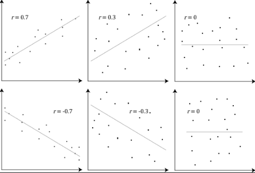
It is a corollary of the Cauchy–Schwarz inequality that the absolute value of the Pearson correlation coefficient is not bigger than 1. Therefore, the value of a correlation coefficient ranges between -1 and +1. The correlation coefficient is +1 in the case of a perfect direct (increasing) linear relationship (correlation), −1 in the case of a perfect inverse (decreasing) linear relationship (anti-correlation),[2] and some value in the open interval [math]\displaystyle{ (-1,1) }[/math] in all other cases, indicating the degree of linear dependence between the variables. As it approaches zero there is less of a relationship (closer to uncorrelated). The closer the coefficient is to either −1 or 1, the stronger the correlation between the variables.
If the variables are independent, Pearson's correlation coefficient is 0, but the converse is not true because the correlation coefficient detects only linear dependencies between two variables.
[math]\displaystyle{ \begin{align} X,Y \text{ independent} \quad & \Rightarrow \quad \rho_{X,Y} = 0 \quad (X,Y \text{ uncorrelated})\\ \rho_{X,Y} = 0 \quad (X,Y \text{ uncorrelated})\quad & \nRightarrow \quad X,Y \text{ independent} \end{align} }[/math]
For example, suppose the random variable [math]\displaystyle{ X }[/math] is symmetrically distributed about zero, and [math]\displaystyle{ Y=X^2 }[/math]. Then [math]\displaystyle{ Y }[/math] is completely determined by [math]\displaystyle{ X }[/math], so that [math]\displaystyle{ X }[/math] and [math]\displaystyle{ Y }[/math] are perfectly dependent, but their correlation is zero; they are uncorrelated. However, in the special case when [math]\displaystyle{ X }[/math] and [math]\displaystyle{ Y }[/math] are jointly normal, uncorrelatedness is equivalent to independence.
Even though uncorrelated data does not necessarily imply independence, one can check if random variables are independent if their mutual information is 0.
1.4. Sample Correlation Coefficient
Given a series of [math]\displaystyle{ n }[/math] measurements of the pair [math]\displaystyle{ (X_i,Y_i) }[/math] indexed by [math]\displaystyle{ i=1,\ldots,n }[/math], the sample correlation coefficient can be used to estimate the population Pearson correlation [math]\displaystyle{ \rho_{X,Y} }[/math] between [math]\displaystyle{ X }[/math] and [math]\displaystyle{ Y }[/math]. The sample correlation coefficient is defined as
- [math]\displaystyle{ r_{xy} \quad \overset{\underset{\mathrm{def}}{}}{=} \quad \frac{\sum\limits_{i=1}^n (x_i-\bar{x})(y_i-\bar{y})}{(n-1)s_x s_y} =\frac{\sum\limits_{i=1}^n (x_i-\bar{x})(y_i-\bar{y})} {\sqrt{\sum\limits_{i=1}^n (x_i-\bar{x})^2 \sum\limits_{i=1}^n (y_i-\bar{y})^2}}, }[/math]
where [math]\displaystyle{ \overline{x} }[/math] and [math]\displaystyle{ \overline{y} }[/math] are the sample means of [math]\displaystyle{ X }[/math] and [math]\displaystyle{ Y }[/math], and [math]\displaystyle{ s_x }[/math] and [math]\displaystyle{ s_y }[/math] are the corrected sample standard deviations of [math]\displaystyle{ X }[/math] and [math]\displaystyle{ Y }[/math].
Equivalent expressions for [math]\displaystyle{ r_{xy} }[/math] are
- [math]\displaystyle{ \begin{align} r_{xy} &=\frac{\sum x_iy_i-n \bar{x} \bar{y}}{n s'_x s'_y} \\[5pt] &=\frac{n\sum x_iy_i-\sum x_i\sum y_i}{\sqrt{n\sum x_i^2-(\sum x_i)^2}~\sqrt{n\sum y_i^2-(\sum y_i)^2}}. \end{align} }[/math]
where [math]\displaystyle{ s'_x }[/math] and [math]\displaystyle{ s'_y }[/math] are the uncorrected sample standard deviations of [math]\displaystyle{ X }[/math] and [math]\displaystyle{ Y }[/math].
If [math]\displaystyle{ x }[/math] and [math]\displaystyle{ y }[/math] are results of measurements that contain measurement error, the realistic limits on the correlation coefficient are not −1 to +1 but a smaller range.[3] For the case of a linear model with a single independent variable, the coefficient of determination (R squared) is the square of [math]\displaystyle{ r_{xy} }[/math], Pearson's product-moment coefficient.
2. Example
Consider the joint probability distribution of [math]\displaystyle{ X }[/math] and [math]\displaystyle{ Y }[/math] given in the table below.
| [math]\displaystyle{ \operatorname{P}(X=x,Y=y) }[/math] | [math]\displaystyle{ y=-1 }[/math] | [math]\displaystyle{ y=0 }[/math] | [math]\displaystyle{ y=1 }[/math] |
| [math]\displaystyle{ x=0 }[/math] | [math]\displaystyle{ 0 }[/math] | [math]\displaystyle{ 1/3 }[/math] | [math]\displaystyle{ 0 }[/math] |
| [math]\displaystyle{ x=1 }[/math] | [math]\displaystyle{ 1/3 }[/math] | [math]\displaystyle{ 0 }[/math] | [math]\displaystyle{ 1/3 }[/math] |
For this joint distribution, the marginal distributions are:
- [math]\displaystyle{ \operatorname{P}(X=x)= \begin{cases} 1/3 & \quad \text{for } x=0 \\ 2/3 & \quad \text{for } x=1 \end{cases} }[/math]
- [math]\displaystyle{ \operatorname{P}(Y=y)= \begin{cases} 1/3 & \quad \text{for } y=-1 \\ 1/3 & \quad \text{for } y=0 \\ 1/3 & \quad \text{for } y=1 \end{cases} }[/math]
This yields the following expectations and variances:
- [math]\displaystyle{ \mu_X = 2/3 }[/math]
- [math]\displaystyle{ \mu_Y = 0 }[/math]
- [math]\displaystyle{ \sigma_X^2 = 2/9 }[/math]
- [math]\displaystyle{ \sigma_Y^2 = 2/3 }[/math]
Therefore:
- [math]\displaystyle{ \begin{align} \rho_{X,Y} & = \frac{1}{\sigma_X \sigma_Y} \operatorname{E}[(X-\mu_X)(Y-\mu_Y)] \\[5pt] & = \frac{1}{\sigma_X \sigma_Y} \sum_{x,y}{(x-\mu_X)(y-\mu_Y) \operatorname{P}(X=x,Y=y)} \\[5pt] & = (1-2/3)(-1-0)\frac{1}{3} + (0-2/3)(0-0)\frac{1}{3} + (1-2/3)(1-0)\frac{1}{3} = 0. \end{align} }[/math]
3. Rank Correlation Coefficients
Rank correlation coefficients, such as Spearman's rank correlation coefficient and Kendall's rank correlation coefficient (τ) measure the extent to which, as one variable increases, the other variable tends to increase, without requiring that increase to be represented by a linear relationship. If, as the one variable increases, the other decreases, the rank correlation coefficients will be negative. It is common to regard these rank correlation coefficients as alternatives to Pearson's coefficient, used either to reduce the amount of calculation or to make the coefficient less sensitive to non-normality in distributions. However, this view has little mathematical basis, as rank correlation coefficients measure a different type of relationship than the Pearson product-moment correlation coefficient, and are best seen as measures of a different type of association, rather than as an alternative measure of the population correlation coefficient.[4][5]
To illustrate the nature of rank correlation, and its difference from linear correlation, consider the following four pairs of numbers [math]\displaystyle{ (x,y) }[/math]:
- (0, 1), (10, 100), (101, 500), (102, 2000).
As we go from each pair to the next pair [math]\displaystyle{ x }[/math] increases, and so does [math]\displaystyle{ y }[/math]. This relationship is perfect, in the sense that an increase in [math]\displaystyle{ x }[/math] is always accompanied by an increase in [math]\displaystyle{ y }[/math]. This means that we have a perfect rank correlation, and both Spearman's and Kendall's correlation coefficients are 1, whereas in this example Pearson product-moment correlation coefficient is 0.7544, indicating that the points are far from lying on a straight line. In the same way if [math]\displaystyle{ y }[/math] always decreases when [math]\displaystyle{ x }[/math] increases, the rank correlation coefficients will be −1, while the Pearson product-moment correlation coefficient may or may not be close to −1, depending on how close the points are to a straight line. Although in the extreme cases of perfect rank correlation the two coefficients are both equal (being both +1 or both −1), this is not generally the case, and so values of the two coefficients cannot meaningfully be compared.[4] For example, for the three pairs (1, 1) (2, 3) (3, 2) Spearman's coefficient is 1/2, while Kendall's coefficient is 1/3.
4. Other Measures of Dependence Among Random Variables
The information given by a correlation coefficient is not enough to define the dependence structure between random variables.[6] The correlation coefficient completely defines the dependence structure only in very particular cases, for example when the distribution is a multivariate normal distribution. (See diagram above.) In the case of elliptical distributions it characterizes the (hyper-)ellipses of equal density; however, it does not completely characterize the dependence structure (for example, a multivariate t-distribution's degrees of freedom determine the level of tail dependence).
Distance correlation[7][8] was introduced to address the deficiency of Pearson's correlation that it can be zero for dependent random variables; zero distance correlation implies independence.
The Randomized Dependence Coefficient[9] is a computationally efficient, copula-based measure of dependence between multivariate random variables. RDC is invariant with respect to non-linear scalings of random variables, is capable of discovering a wide range of functional association patterns and takes value zero at independence.
For two binary variables, the odds ratio measures their dependence, and takes range non-negative numbers, possibly infinity: [math]\displaystyle{ [0, +\infty] }[/math]. Related statistics such as Yule's Y and Yule's Q normalize this to the correlation-like range [math]\displaystyle{ [-1, 1] }[/math]. The odds ratio is generalized by the logistic model to model cases where the dependent variables are discrete and there may be one or more independent variables.
The correlation ratio, entropy-based mutual information, total correlation, dual total correlation and polychoric correlation are all also capable of detecting more general dependencies, as is consideration of the copula between them, while the coefficient of determination generalizes the correlation coefficient to multiple regression.
5. Sensitivity to the Data Distribution
The degree of dependence between variables [math]\displaystyle{ X }[/math] and [math]\displaystyle{ Y }[/math] does not depend on the scale on which the variables are expressed. That is, if we are analyzing the relationship between [math]\displaystyle{ X }[/math] and [math]\displaystyle{ Y }[/math], most correlation measures are unaffected by transforming [math]\displaystyle{ X }[/math] to a + bX and [math]\displaystyle{ Y }[/math] to c + dY, where a, b, c, and d are constants (b and d being positive). This is true of some correlation statistics as well as their population analogues. Some correlation statistics, such as the rank correlation coefficient, are also invariant to monotone transformations of the marginal distributions of [math]\displaystyle{ X }[/math] and/or [math]\displaystyle{ Y }[/math].
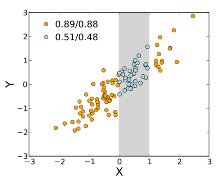
Most correlation measures are sensitive to the manner in which [math]\displaystyle{ X }[/math] and [math]\displaystyle{ Y }[/math] are sampled. Dependencies tend to be stronger if viewed over a wider range of values. Thus, if we consider the correlation coefficient between the heights of fathers and their sons over all adult males, and compare it to the same correlation coefficient calculated when the fathers are selected to be between 165 cm and 170 cm in height, the correlation will be weaker in the latter case. Several techniques have been developed that attempt to correct for range restriction in one or both variables, and are commonly used in meta-analysis; the most common are Thorndike's case II and case III equations.[10]
Various correlation measures in use may be undefined for certain joint distributions of X and Y. For example, the Pearson correlation coefficient is defined in terms of moments, and hence will be undefined if the moments are undefined. Measures of dependence based on quantiles are always defined. Sample-based statistics intended to estimate population measures of dependence may or may not have desirable statistical properties such as being unbiased, or asymptotically consistent, based on the spatial structure of the population from which the data were sampled.
Sensitivity to the data distribution can be used to an advantage. For example, scaled correlation is designed to use the sensitivity to the range in order to pick out correlations between fast components of time series.[11] By reducing the range of values in a controlled manner, the correlations on long time scale are filtered out and only the correlations on short time scales are revealed.
6. Correlation Matrices
The correlation matrix of [math]\displaystyle{ n }[/math] random variables [math]\displaystyle{ X_1,\ldots,X_n }[/math] is the [math]\displaystyle{ n \times n }[/math] matrix whose [math]\displaystyle{ (i,j) }[/math] entry is [math]\displaystyle{ \operatorname{corr}(X_i,X_j) }[/math]. Thus the diagonal entries are all identically unity. If the measures of correlation used are product-moment coefficients, the correlation matrix is the same as the covariance matrix of the standardized random variables [math]\displaystyle{ X_i / \sigma(X_i) }[/math] for [math]\displaystyle{ i = 1, \dots, n }[/math]. This applies both to the matrix of population correlations (in which case [math]\displaystyle{ \sigma }[/math] is the population standard deviation), and to the matrix of sample correlations (in which case [math]\displaystyle{ \sigma }[/math] denotes the sample standard deviation). Consequently, each is necessarily a positive-semidefinite matrix. Moreover, the correlation matrix is strictly positive definite if no variable can have all its values exactly generated as a linear function of the values of the others.
The correlation matrix is symmetric because the correlation between [math]\displaystyle{ X_i }[/math] and [math]\displaystyle{ X_j }[/math] is the same as the correlation between [math]\displaystyle{ X_j }[/math] and [math]\displaystyle{ X_i }[/math].
A correlation matrix appears, for example, in one formula for the coefficient of multiple determination, a measure of goodness of fit in multiple regression.
In statistical modelling, correlation matrices representing the relationships between variables are categorized into different correlation structures, which are distinguished by factors such as the number of parameters required to estimate them. For example, in an exchangeable correlation matrix, all pairs of variables are modeled as having the same correlation, so all non-diagonal elements of the matrix are equal to each other. On the other hand, an autoregressive matrix is often used when variables represent a time series, since correlations are likely to be greater when measurements are closer in time. Other examples include independent, unstructured, M-dependent, and Toeplitz.
7. Nearest Valid Correlation Matrix
In some applications (e.g., building data models from only partially observed data) one wants to find the "nearest" correlation matrix to an "approximate" correlation matrix (e.g., a matrix which typically lacks semi-definite positiveness due to the way it has been computed).
In 2002, Higham[12] formalized the notion of nearness using the Frobenius norm and provided a method for computing the nearest correlation matrix using the Dykstra's projection algorithm, of which an implementation is available as an online Web API.[13]
This sparked interest in the subject, with new theoretical (e.g., computing the nearest correlation matrix with factor structure[14]) and numerical (e.g. usage the Newton's method for computing the nearest correlation matrix[15]) results obtained in the subsequent years.
Similarly for two stochastic processes [math]\displaystyle{ \left\{ X_t \right\}_{t\in\mathcal{T}} }[/math] and [math]\displaystyle{ \left\{ Y_t \right\}_{t\in\mathcal{T}} }[/math]: If they are independent, then they are uncorrelated.[16]:p. 151
9. Common Misconceptions
9.1. Correlation and Causality
The conventional dictum that "correlation does not imply causation" means that correlation cannot be used by itself to infer a causal relationship between the variables.[17] This dictum should not be taken to mean that correlations cannot indicate the potential existence of causal relations. However, the causes underlying the correlation, if any, may be indirect and unknown, and high correlations also overlap with identity relations (tautologies), where no causal process exists. Consequently, a correlation between two variables is not a sufficient condition to establish a causal relationship (in either direction).
A correlation between age and height in children is fairly causally transparent, but a correlation between mood and health in people is less so. Does improved mood lead to improved health, or does good health lead to good mood, or both? Or does some other factor underlie both? In other words, a correlation can be taken as evidence for a possible causal relationship, but cannot indicate what the causal relationship, if any, might be.
9.2. Simple Linear Correlations
The Pearson correlation coefficient indicates the strength of a linear relationship between two variables, but its value generally does not completely characterize their relationship.[18] In particular, if the conditional mean of [math]\displaystyle{ Y }[/math] given [math]\displaystyle{ X }[/math], denoted [math]\displaystyle{ \operatorname{E}(Y \mid X) }[/math], is not linear in [math]\displaystyle{ X }[/math], the correlation coefficient will not fully determine the form of [math]\displaystyle{ \operatorname{E}(Y \mid X) }[/math].
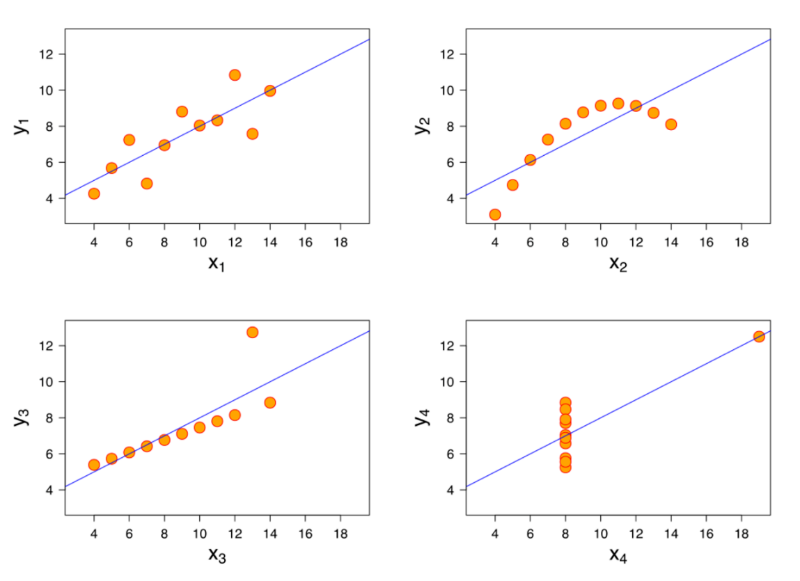
The adjacent image shows scatter plots of Anscombe's quartet, a set of four different pairs of variables created by Francis Anscombe.[19] The four [math]\displaystyle{ y }[/math] variables have the same mean (7.5), variance (4.12), correlation (0.816) and regression line (y = 3 + 0.5x). However, as can be seen on the plots, the distribution of the variables is very different. The first one (top left) seems to be distributed normally, and corresponds to what one would expect when considering two variables correlated and following the assumption of normality. The second one (top right) is not distributed normally; while an obvious relationship between the two variables can be observed, it is not linear. In this case the Pearson correlation coefficient does not indicate that there is an exact functional relationship: only the extent to which that relationship can be approximated by a linear relationship. In the third case (bottom left), the linear relationship is perfect, except for one outlier which exerts enough influence to lower the correlation coefficient from 1 to 0.816. Finally, the fourth example (bottom right) shows another example when one outlier is enough to produce a high correlation coefficient, even though the relationship between the two variables is not linear.
These examples indicate that the correlation coefficient, as a summary statistic, cannot replace visual examination of the data. The examples are sometimes said to demonstrate that the Pearson correlation assumes that the data follow a normal distribution, but this is not correct.[1]
10. Bivariate Normal Distribution
If a pair [math]\displaystyle{ (X,Y) }[/math] of random variables follows a bivariate normal distribution, the conditional mean [math]\displaystyle{ \operatorname{E}(X \mid Y) }[/math] is a linear function of [math]\displaystyle{ Y }[/math], and the conditional mean [math]\displaystyle{ \operatorname{E}(Y \mid X) }[/math] is a linear function of [math]\displaystyle{ X }[/math]. The correlation coefficient [math]\displaystyle{ \rho_{X,Y} }[/math] between [math]\displaystyle{ X }[/math] and [math]\displaystyle{ Y }[/math], along with the marginal means and variances of [math]\displaystyle{ X }[/math] and [math]\displaystyle{ Y }[/math], determines this linear relationship:
- [math]\displaystyle{ \operatorname{E}(Y\mid X) = \operatorname{E}(Y) + \rho_{X,Y} \cdot \sigma_Y\frac{X-\operatorname{E}(X)}{\sigma_X}, }[/math]
where [math]\displaystyle{ \operatorname{E}(X) }[/math] and [math]\displaystyle{ \operatorname{E}(Y) }[/math] are the expected values of [math]\displaystyle{ X }[/math] and [math]\displaystyle{ Y }[/math], respectively, and [math]\displaystyle{ \sigma_X }[/math] and [math]\displaystyle{ \sigma_Y }[/math] are the standard deviations of [math]\displaystyle{ X }[/math] and [math]\displaystyle{ Y }[/math], respectively.
References
- Rodgers, J. L.; Nicewander, W. A. (1988). "Thirteen ways to look at the correlation coefficient". The American Statistician 42 (1): 59–66. doi:10.1080/00031305.1988.10475524. https://dx.doi.org/10.1080%2F00031305.1988.10475524
- Dowdy, S. and Wearden, S. (1983). "Statistics for Research", Wiley. ISBN:0-471-08602-9 pp 230
- Francis, DP; Coats AJ; Gibson D (1999). "How high can a correlation coefficient be?". Int J Cardiol 69 (2): 185–199. doi:10.1016/S0167-5273(99)00028-5. https://dx.doi.org/10.1016%2FS0167-5273%2899%2900028-5
- Yule, G.U and Kendall, M.G. (1950), "An Introduction to the Theory of Statistics", 14th Edition (5th Impression 1968). Charles Griffin & Co. pp 258–270
- Kendall, M. G. (1955) "Rank Correlation Methods", Charles Griffin & Co.
- Mahdavi Damghani B. (2013). "The Non-Misleading Value of Inferred Correlation: An Introduction to the Cointelation Model". Wilmott Magazine 2013 (67): 50–61. doi:10.1002/wilm.10252. https://dx.doi.org/10.1002%2Fwilm.10252
- Székely, G. J. Rizzo; Bakirov, N. K. (2007). "Measuring and testing independence by correlation of distances". Annals of Statistics 35 (6): 2769–2794. doi:10.1214/009053607000000505. https://dx.doi.org/10.1214%2F009053607000000505
- Székely, G. J.; Rizzo, M. L. (2009). "Brownian distance covariance". Annals of Applied Statistics 3 (4): 1233–1303. doi:10.1214/09-AOAS312. PMID 20574547. http://www.pubmedcentral.nih.gov/articlerender.fcgi?tool=pmcentrez&artid=2889501
- Lopez-Paz D. and Hennig P. and Schölkopf B. (2013). "The Randomized Dependence Coefficient", "Conference on Neural Information Processing Systems" Reprint http://papers.nips.cc/paper/5138-the-randomized-dependence-coefficient.pdf
- Thorndike, Robert Ladd (1947). Research problems and techniques (Report No. 3). Washington DC: US Govt. print. off..
- Nikolić, D; Muresan, RC; Feng, W; Singer, W (2012). "Scaled correlation analysis: a better way to compute a cross-correlogram". European Journal of Neuroscience 35 (5): 1–21. doi:10.1111/j.1460-9568.2011.07987.x. PMID 22324876. https://dx.doi.org/10.1111%2Fj.1460-9568.2011.07987.x
- Higham, Nicholas J. (2002). "Computing the nearest correlation matrix—a problem from finance". IMA Journal of Numerical Analysis 22 (3): 329–343. doi:10.1093/imanum/22.3.329. https://dx.doi.org/10.1093%2Fimanum%2F22.3.329
- "Portfolio Optimizer". https://portfoliooptimizer.io/.
- Borsdorf, Rudiger; Higham, Nicholas J.; Raydan, Marcos (2010). "Computing a Nearest Correlation Matrix with Factor Structure.". SIAM J. Matrix Anal. Appl. 31 (5): 2603–2622. doi:10.1137/090776718. https://dx.doi.org/10.1137%2F090776718
- Qi, HOUDUO; Sun, DEFENG (2006). "A quadratically convergent Newton method for computing the nearest correlation matrix.". SIAM J. Matrix Anal. Appl. 28 (2): 360–385. doi:10.1137/050624509. https://dx.doi.org/10.1137%2F050624509
- Park, Kun Il (2018). Fundamentals of Probability and Stochastic Processes with Applications to Communications. Springer. ISBN 978-3-319-68074-3.
- Aldrich, John (1995). "Correlations Genuine and Spurious in Pearson and Yule". Statistical Science 10 (4): 364–376. doi:10.1214/ss/1177009870. https://dx.doi.org/10.1214%2Fss%2F1177009870
- Mahdavi Damghani, Babak (2012). "The Misleading Value of Measured Correlation". Wilmott Magazine 2012 (1): 64–73. doi:10.1002/wilm.10167. https://dx.doi.org/10.1002%2Fwilm.10167
- Anscombe, Francis J. (1973). "Graphs in statistical analysis". The American Statistician 27 (1): 17–21. doi:10.2307/2682899. https://dx.doi.org/10.2307%2F2682899

