1. Naming in Other Parts of the World

In other regions the glaciations of the last glacial period are given other names: for example that in the Alpine region is called the Würm glaciation, in Great Britain it is the Devensian glaciation, in Ireland the Midlandian glaciation and in North America, the Wisconsin glaciation.^[1][2]

2. Development of the Glaciation

2.1. Early and Middle Weichselian

The Fennoscandian Ice Sheet of the Weichselian glaciation most likely grew out of a mountain glaciation of small ice fields and ice caps in the Scandinavian Mountains. The initial glaciation of the Scandinavian Mountains would have been enabled by moisture coming from the Atlantic Ocean and the mountains high altitude. Perhaps the best modern analogues to this early glaciation are the ice fields of Andean Patagonia.^[3]

Jan Mangerud posits that parts of the Norwegian coast were likely free from glacier ice during most of the Weichselian prior to the Last Glacial Maximum.^[4]

Between 38 and 28 ka BP there was a relatively warm period in Fennoscandia called the Ålesund interstadial. The interstadial receives its name from the Ålesund municipality in Norway where its existence was first established based on the local fossil record of shells.^[5]

2.2. Last Glacial Maximum

Template:FarblegendeTemplate:Farblegende Note that the coastlines are modern; coastlines during the Weichselian were different as sea level was lower. By The original uploader was Fice at German Wikipedia. - Eigene Graphik auf der Grundlage der Wikipedia-Abbildung de:Bild:Deutschland topo.jpg (Ausschnitt)., CC BY-SA 3.0, https://commons.wikimedia.org/w/index.php?curid=5524035

The growth of the ice sheet to its Last Glacial Maximum extent begun after the Ålesund interstadial.^[6]

The growth of the ice sheet was accompanied by an eastward migration of the ice divide from the Scandinavian Mountains eastwards into Sweden and the Baltic Sea.^[7] As the ice sheets in northern Europe grew prior to the Last Glacial Maximum the Fennoscandian Ice sheet coalesced with the ice sheet that was growing in Barents Sea 24 ka BP (kiloannus or one thousand years Before Present) and with the ice sheet of the British Islands at about thousand years later. At this point the Fennoscandian Ice Sheet formed part of a larger Eurasian ice sheet complex—a contiguous glacial ice mass which spanned an area from Ireland to Novaya Zemlya.^[7]

The central parts of the Weichsel ice sheet had cold-based conditions during the times of maximum extent. This means that in areas like north-east Sweden and northern Finland pre-existing landforms and deposits escaped glacier erosion and are particularly well preserved at present.^[8] Also during times of maximum extent the ice sheet terminated to the east in a gently uphill terrain meaning that rivers drained into the glacier front and large proglacial lakes built up.^[6]

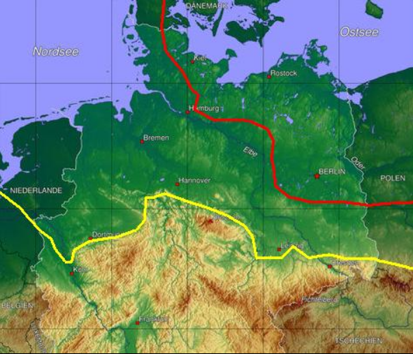
The Last Glacial Maximum extent was first reached 22 ka BP in the southern boundary of the ice sheet in Denmark, Germany and Western Poland. In Eastern Poland, Lithuania, Belarus and Pskov Oblast in Russia the ice sheet reached its maximum extent about 19 ka BP. In the remainder of northwestern Russia the largest glacier advance occurred 17 ka BP.^[9]

2.3. Deglaciation up to Younger Dryas

As the ice margin started to recede 22-17 ka BP Denmark (except Bornholm), Germany, Poland and Belarus were ice-free 16 ka BP. The ice margin then retreated until the Younger Dryas when the ice sheet stabilized. By this time, most of Götaland, Gotland, all of the Baltic states and the southeastern coast of Finland had been added to the ice-free regions. In Russia, Lake Ladoga, Lake Onega, the bulk of Kola Peninsula and the White Sea were free from ice during the Younger Dryas. Before the Younger Dryas, deglaciation had not been uniform and small ice sheet re-advances had occurred forming a series of end-moraine systems, notably those in Götaland.^[9]

During deglaciation, meltwater formed numerous eskers and sandurs. In north-central Småland and southern Östergötland part of the meltwater was routed through a series of canyons.^[10]

It is speculated that during the Younger Dryas a small glacier readvance in Sweden created a natural lock system that brought freshwater taxa such as Mysis and Salvelinus to lakes like Sommen that were never connected to the Baltic Ice Lake. The survival of these cold-water taxa into the present-day means they are glacial relicts.^[11][12]

2.4. Final deglaciation

When ice margin retreat resumed the ice sheet became increasingly concentrated in the Scandinavian Mountains (it had left Russia 10.6 ka BP and Finland 10.1 ka BP). Further retreat of the ice margin led the ice sheet to concentrate in two parts of the Scandinavian Mountains, one part in Southern Norway and another in Northern Sweden and Norway. These two centres were linked for a time. The linkage constituted a major drainage barrier that formed various large and ephemeral ice-dammed lakes. About 10.1 ka BP the linkage had disappeared and so did the Southern Norway centre of the ice sheet about a thousand years later. The northern centre remained a few hundred years more so that by 9.7 ka BP the eastern Sarek Mountains hosted the last remnant of the Fennoscandian Ice Sheet.^[9] As the ice sheet retreated to the Scandinavian Mountains this was not a return to its former mountain centred glaciation from which the ice sheet grew out, it was dissimilar in that the ice divide lagged behind as the ice mass concentrated in the west.^[3]

It is not known if the if the ice sheet disintegrated into scattered remains before vanishing or if it shrunk while maintaining its coherence as a single ice mass.^[13] It is possible that while some ice remained east of Sarek Mountains parts of the ice sheet survived temporarily in the high mountains.^[13] Remnants east of the Sarek Mountains formed various ephemeral ice-dammed lakes that caused numerous glacial lake outburst floods down the rivers of northernmost Sweden.^[13]

2.5. Isostatic adjustment

Map of the Littorina Sea around 7000 years BP. Note the reduced area of Finland due to higher sea levels.

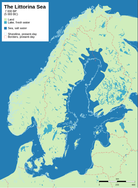
Isostatic adjustment bought by deglaciation is reflected in the shoreline changes of the Baltic Sea and other nearby bodies of water.^[14] In the Baltic Sea uplift has been greatest at the High Coast in the western Bothnian Sea. Within the High Coast the relict shoreline at 286 m in Skuleberget is at present the highest known point on Earth to have been uplifted by postglacial isostatic rebound.^[15] North of the High Coast at Furuögrund off the coast of Skellefteå lies the area with the highest uplift rates at present with values of about 9 mm/yr.^[15][16][17] Ongoing post-glacial rebound is thought to result in splitting of the Gulf of Bothnia into a southern gulf and a northern lake across Norra Kvarken no earlier than in about 2,000 years.^[18] Isostatic rebound exposed a submarine joint valley landscape as Stockholm archipelago.^[19][20]

Since deglaciation the rate of post-glacial rebound in the Kandalaksha Gulf has varied. Since the White Sea connected to the world's oceans uplift along the southern coast of the gulf has totaled 90 m. In the interval from 9,500–5,000 years ago the uplift rate was of 9–13 mm/yr. Prior to the Atlantic period the uplift rate had decreased to 5–5.5 mm/yr, to then rose briefly before arriving at the present uplift rate of 4 mm/yr.^[21]

Emergence above sea level is thought to have resulted in the triggering of a series of landslides in western Sweden as pore pressure increased when the groundwater recharge zone came above sea level.^[22]

3. Sequence and Subdivisions of the Weichselian

Depiction of the Earth at the last glacial maximum. Illustration based on: Ice age terrestrial carbon changes revisited by Thomas J. Crowley (Global Biogeochemical Cycles, Vol. 9, 1995, pp. 377-389). By Ittiz - Own work, CC BY-SA 3.0, https://commons.wikimedia.org/w/index.php?curid=9237442

About 115,000 years ago^[23] average temperatures dropped markedly and warmth-loving woodland species were displaced. This significant turning point in average temperatures marked the end of the Eemian interglacial and start of the Weichselian glacial stage. It is divided into three sections, based on the temperature variation: the Weichselian Early Glacial,^[24][25] the Weichselian High Glacial^[24] (also Weichselian Pleniglacial^[25]) and the Weichselian Late Glacial.^[25] During the Weichselian, there were frequent major variations in climate in the northern hemisphere, the so-called Dansgaard-Oeschger events.

The Weichsel Early Glacial (115,000 - 60,000 BC) is in turn divided into four stages:

• Odderade Interstadial (WF IV) - The pollen spectra indicate a boreal forest. It starts with a tree birch phase, which rapidly transitions to pine forest. Also apparent are larches and spruce as well as low numbers of alder.
• Rederstall Stadial (also WF III) - In North Germany the pollen spectra indicate a grassy tundra followed later by shrubby tundra.
• Brörup Interstadial (also WF II) - Several profiles show a short period of cooling shortly after the start of the Brörup Interstadial, but this does not appear in all profiles. This led some authors to distinguish the first warm period as the Amersfoort Interstadial. However, since then, this first warm period and cooling phase has been included in the Brörup Interstadial. Northern Central Europe was populated by birch and pine woods. The Brörup Interstadial is identified with marine isotope stage 5c.
• Herning Stadial (also called WF I) - Was the first cold phase, in which northwestern Europe was largely treeless. It corresponds to marine isotope stage 5d.

In the Weichselian High Glacial (57,000 - c. 15,000 BC) the ice sheet advanced into North Germany. In this period, however, several interstadials have been documented.

• Glaciation and ice sheet advances to North Germany (Brandenburg Phase, Frankfurt Phase, Pomeranian Phase, Mecklenburg Phase).
• Denekamp Interstadial - The pollen spectra indicates a shrubby tundra landscape.
• Hengelo Interstadial - The pollen show sedges (Cyperaceae) and temporarily a high number of dwarf birches (Betula nana).
• Moershoofd Interstadial - The pollen spectra show a treeless tundra vegetation with a high proportion of sedges (Cyperaceae).
• Glinde Interstadial (WP IV) - The pollen diagrams indicate a treeless, shrubby tundra.
• Ebersdorf Stadial (WP III) - In North Germany this period is characterised by pollen-free sands.
• Oerel Interstadial (WP II) - The pollen diagrams point to a treeless, shrubby tundra in North Germany.
• Schalkholz Stadial (WP I) - The first ice advance may have already reached the southern Baltic Sea coast. At the type locality of Schalkholz (county of Dithmarschen) pollen-free, sands indicate a largely vegetation-free landscape.

The short "Weichselian Late Glacial" (12,500 - c. 10,000 BC) was the period of slow warming after the Weichselian High Glacial. It was however again interrupted by some colder episodes.

• Younger Dryas - In this period the proportion of non-tree pollens climbed again, especially those of heliophytes.
• Allerød oscillation - This section is again dominated by birch tree pollens.
• Older Dryas - This cool period is characterised by a reduction in tree pollens.
• Bølling oscillation - The period begins with a rapid increase in tree birch pollens.
• Oldest Dryas - The cool period is characterised by a maximum number of non-tree pollens.
• Meiendorf Interstadial - This interstadial is typified by a rise in the pollens of dwarf birches (Betula nana), willows (Salix sp.), sandthorns (Hippophae), junipers (Juniperus) and sagebrush (Artemisia).

Following the last of these cold periods, the Younger Dryas, the Weichselian Glacial ended with an abrupt climb in temperature around 9,660 ± 40 BC.^[26] This was the start of our present interglacial, the Holocene.

In addition to the above subdivisions the depositions of the Weichselian Late Glacial following the retreat of the ice sheet are divided into four stages: the Germanic Glacial (Germaniglazial) (Germany becomes ice-free), the Danish Glacial (Daniglazial) (Denmark becomes ice-free), The Gotland Glacial (Gotiglazial) (Gotland becomes ice-free) and the Finnish Glacial (Finiglazial) (Finland and Norway become ice-free).^[27]

References

- F.J. Monkhouse Principles of Physical Geography, London: University of London Press, 1970 (7th edn.), p. 254. SBN 340 09022 7
- Whittow, John (1984). Dictionary of Physical Geography. London: Penguin, 1984, p. 265. ISBN:0-14-051094-X.
- "Glacial inception and Quaternary mountain glaciations in Fennoscandia". Quaternary International 95–96: 99–112. 2002. doi:10.1016/s1040-6182(02)00031-9. Bibcode: 2002QuInt..95...99F. https://dx.doi.org/10.1016%2Fs1040-6182%2802%2900031-9
- Mangerud, Jan (1981). "The Early and Middle Weichselian in Norway: a review". Boreas 10 (4): 447–462. doi:10.1111/j.1502-3885.1981.tb00508.x. https://dx.doi.org/10.1111%2Fj.1502-3885.1981.tb00508.x
- Mangerud, Jan; Gulliksen, Steinar; Larsen, Eiliv; Oddvar, Longva; Miller, Gifford H.; Sejrup, Hans-Petter; Sønstegaard, Eivind (1981). "A Middle Weichselain ice-free period in Western Norway: the Ålesund Interstadial". Boreas 10 (4): 381–393. doi:10.1111/j.1502-3885.1981.tb00500.x. https://dx.doi.org/10.1111%2Fj.1502-3885.1981.tb00500.x
- Larsen, Eiliv; Fredin, Ola; Lyså, Astrid; Amantov, Aleksey; Feldskaar, Willy; Ottesen, Dag (2016). "Causes of time-transgressive glacial maxima positions of the last Scandinavian Ice Sheet". Norwegian Journal of Geology 96 (2): 159–170. http://njg.geologi.no/images/NJG_articles/NJG_Vol96_No2_Article6_Larsen_etal.pdf. Retrieved January 20, 2018.
- Patton, Henry; Hubbard, Alun; Andreasen, Karin; Auriac, Amandine; Whitehouse, Pippa L.; Stroeven, Arjen P.; Shackleton, Calvin; Winsborrow, Monica et al. (2017). "Deglaciation of the Eurasian ice sheet complex". Quaternary Science Reviews 169: 148–172. doi:10.1016/j.quascirev.2017.05.019. Bibcode: 2017QSRv..169..148P. https://dx.doi.org/10.1016%2Fj.quascirev.2017.05.019
- Sarala, Pertti (2005). "Weichselian stratigraphy, geomorphology and glacial dynamics in southern Finnish Lapland". Bulletin of the Geological Society of Finland 77 (2): 71–104. doi:10.17741/bgsf/77.2.001. https://dx.doi.org/10.17741%2Fbgsf%2F77.2.001
- Stroeven, Arjen P; Hättestrand, Clas; Kleman, Johan; Heyman, Jakob; Fabel, Derek; Fredin, Ola; Goodfellow, Bradley W; Harbor, Jonathan M et al. (2016). "Deglaciation of Fennoscandia". Quaternary Science Reviews 147: 91–121. doi:10.1016/j.quascirev.2015.09.016. Bibcode: 2016QSRv..147...91S. https://dx.doi.org/10.1016%2Fj.quascirev.2015.09.016
- Olvmo, M. (1992). "Glaciofluvial canyons and their relation to the Late Weiochselian deglaciation in Fennoscandia". Zeitschrift für Geomorphologie 36 (3): 343–363.
- Kinsten, Björn (2010) (in Swedish). De glacialrelikta kräftdjurens utbredning i södra Sverige (Götaland och Svealand) (Report). Länsstyrelsen Blekinge län. pp. 1–19. https://www.lansstyrelsen.se/download/18.2887c5dd16488fe880d55ad0/1537435814356/rapport-2010-7.pdf. Retrieved April 19, 2019.
- In the isolation that followed the Salvelinus species of Sommen evolved into a distinct subspecies called Sommen charr.[14]
- Regnéll, Carl; Mangerud, Jan; Svendsen, John Inge (2019). "Tracing the last remnants of the Scandinavian Ice Sheet: Ice-dammed lakes and a catastrophic outburst flood in northern Sweden". Quaternary Science Reviews 221: 105862. doi:10.1016/j.quascirev.2019.105862. Bibcode: 2019QSRv..22105862R. https://dx.doi.org/10.1016%2Fj.quascirev.2019.105862
- In the late 19th and early 20th century, N. O. Holst (1899), Ernst Antevs (1921) and Astrid Cleve (1923) proposed the so-called oscillation theory, which holds that the land-level had oscillated up and down "like a pendulum losing momentum" after deglaciation. The Geologiska föreningen society expulsed Cleve for her unrelenting support of this theory once it became discredited.[16]
- Berglund, M. (2012). "The highest postglacial shore levels and glacio-isostatic uplift pattern in northern Sweden". Geografiska Annaler: Series A, Physical Geography 94 (3): 321–337. doi:10.1111/j.1468-0459.2011.00443.x. https://dx.doi.org/10.1111%2Fj.1468-0459.2011.00443.x
- Ågren, J. and Svensson, R., 2006. Land uplift model and system definitions used for the RH 2000 adjustment of the Baltic levelling ring. The 15th General Meeting of the Nordic Geodetic Commission, Copenhagen, 29 May–2 June 2006, 1–9
- Davis, J.L.; Mitrovica, J.X.; Scherneck, H.-G.; Fan, H. (1999). "Investigations of Fennoscandian glacial isostatic adjustment using modern sealevel records". Journal of Geophysical Research 104 (B2): 2733–2747. doi:10.1029/1998jb900057. Bibcode: 1999JGR...104.2733D. https://dx.doi.org/10.1029%2F1998jb900057
- Tikkanen, Matti; Oksanen, Juha (2002). "Late Weichselian and Holocene shore displacement history of the Baltic Sea in Finland". Fennia 180 (1–2). http://www.helsinki.fi/maantiede/geofi/fennia/demo/pages/oksanen.htm. Retrieved December 22, 2017.
- Lidmar-Bergströrm, Karna (1995). "Relief and saprolites through time on the Baltic Shield". Geomorphology 12 (1): 45–61. doi:10.1016/0169-555X(94)00076-4. Bibcode: 1995Geomo..12...45L. https://dx.doi.org/10.1016%2F0169-555X%2894%2900076-4
- Sporrong, Ulf (2003). "The Scandinavian landscape and its resources". in Helle, Knut. The Cambridge History of Scandinavia. Cambridge University Press. pp. 37. https://archive.org/details/cambridgehistory01hell.
- Romanenko, F.A.; Shilova, O.S. (2011). "The Postglacial Uplift of the Karelian Coast of the White Sea according to Radiocarbon and Diatom Analyses of LacustrineBoggy Deposits of Kindo Peninsula". Doklady Earth Sciences 442 (2): 544–548. doi:10.1134/S1028334X12020079. Bibcode: 2012DokES.442..242R. https://dx.doi.org/10.1134%2FS1028334X12020079
- Smith, Colby A.; Larsson, Olof; Engdahl, Mats (2017). "Early Holocene coastal landslides linked to land uplift in western Sweden". Geografiska Annaler: Series A, Physical Geography 99 (3): 288–311. doi:10.1080/04353676.2017.1329624. https://dx.doi.org/10.1080%2F04353676.2017.1329624
- Litt et al. (2007: pp.45ff)
- Wolfgang Schirmer, Quaternary field trips in central Europe, Volume 1, Pfeil, 1995, p. 375. ISBN:978-39-238-7191-9
- John Dodson (ed.), Earth Systems and Society, New York, London, etc., Springer, 2010 p. 173. ISBN:978-90-481-8716-4
- Friedrich, M; Kromer, B; Spurk, M; Hofmann, J; Kaiser, KF (1999). "Paleo-environment and radiocarbon calibration as derived from Late Glacial/Early Holocene tree-ring chronologies". Quaternary International 61 (1): 27–39. doi:10.1016/s1040-6182(99)00015-4. Bibcode: 1999QuInt..61...27F. https://dx.doi.org/10.1016%2Fs1040-6182%2899%2900015-4
- Karl N. Thome (1998) (in German), Einführung in das Quartär. Das Zeitalter der Gletscher, Berlin: Springer-Verlag, pp. 72, https://books.google.com/books?id=izM1tK-VtEYC&pg=PA72