Food, Energy and Water Nexus

Version	Summary	Created by	Modification	Content Size	Created at	Operation
1		Maria Ester Soares Dal Poz	--	3489	2022-06-21 16:05:15	\|
2	update layout and references	Rita Xu	Meta information modification	3489	2022-06-22 03:57:00	\|

This entry is adapted from the peer-reviewed paper 10.3390/su14127163

From a climate change perspective, the governance of natural common-pool resources—the commons—is a key point in the challenge of transitioning to sustainability. São Paulo Urban Living Laboratory (ULL) regarding Food, Energy and Water (FEW Nexus) analysis and modelling at the border of a high biodiverse forest in a peri-urban region in southeast Brazil. It is a replicable and scalable method concerning FEW governance. The FEW Nexus is an analytical guide to actions that will enable a colossal set of innovative processes that the transition to sustainability presupposes.

food, energy and water nexus sustainable development

1. Introduction

Climate change—as a phenomenon characteristic of the Anthropocene—is the primary driver of demands for efforts to transition to sustainability. The risk of natural resource scarcity raises a planetary dilemma involving political, social, and economic factors at the macro, meso, and micro-institutional levels, implying systemic changes in markets and modes of production, distribution, marketing, and consumption ^[1]^[2]^[3]^[4].

In this scenario, faith is not enough and action is needed, implementing the process of transition to sustainability, characterised by the almost infinite combination of at least a few thousand factors of production, marketing and consumption behaviour currently in place. The array of combinatorial factors to be considered in the transition is then also nearly infinite ^[5]^[6].

Hence, the search for sustainability proves to be a civilizational milestone, an urgent global collective goal, surrounded by new constitutions and commitments to be undertaken in a highly uncertain process. This is because it implies new patterns of economic production and growth, of developing new markets and adapting old ones, new social relations and consumption behaviour ^[7].

Such a scenario allows researchers to think of the transition as a profound process of evolutionary adaptation regarding the governance of natural common-pool resources, known as commons ^[8]^[9].

Actions that contribute to the transition can thus be seen as the two-faced Janus, the Roman god of changes and transitions, looking at the past and the future, at things as they were and are, and projecting, in foresight, how they could be more sustainable.

This entry presents exemplary research in so-called commons governance towards sustainable food systems (SFS) for food production at the border of the Atlantic Forest, South-eastern Brazil. Although based on a regional SFS case, the sustainability policy support tool is far-reaching, since its structuring governance indicators are applicable to other cases. It is not, in this sense, a single regional or specific decision making tool for development and validation, but a replicable and scalable methodology for FEW governance demands.

The flowchart in Figure 1 illustrates the steps organised in the research.

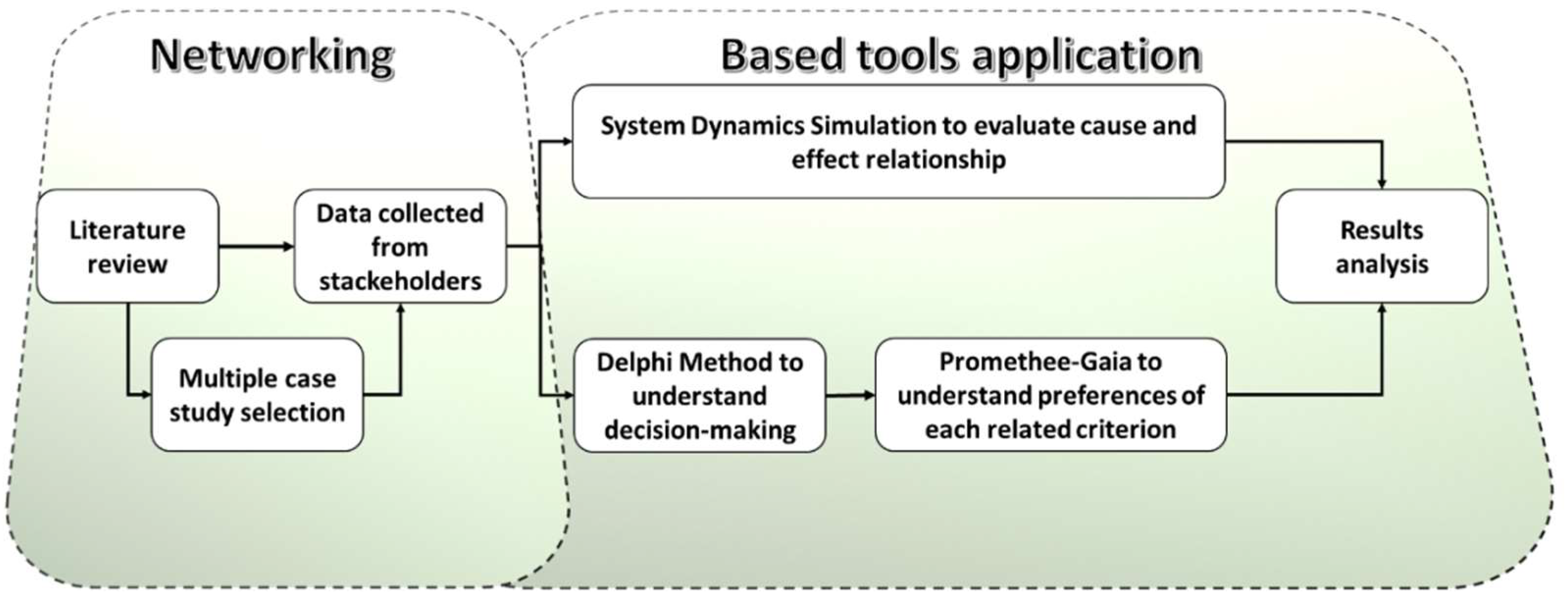
Figure 1. Research design.

Thus, researchers have two layers of analysis, each referring to a core action problem of the Urban Living Laboratory (ULLs), or a Research Question (RQ).

The first RQ is the networking of stakeholders involved in this transition, without whom there is no evolutionary path to change, which is performed by the communities involved in the problem. This community is responsible for characterising the relevant criteria and attributes to guide the transition, resulting in a decision support framework with 13 sustainability indicators that are highly relevant to this process: the Sustainability Policy Innovation Network tool for decision making ^[10].

The second RQ is the application of two tools based on such framework indicators: (a) modelling of complex food production systems, and (b) prospective solution consultation. Conventional and agroecological production systems were researchers' objects of investigation, allowing researchers to understand the relative functionalities and dysfunctionalities of each system, and to identify how the relevant stakeholder communities see the future of the transition process.

2. System Dynamics Modelling: The Backward-Looking Face of Janus

Transition to sustainability comprises a subset of highly complex meta-disciplinary problems. In the case of peri-urban agriculture, such transition requires greater levels of understanding of multi-scale phenomena and common-pool resource use systems.

These are open or semi-open, which makes understanding their dynamics even more uncertain. This aspect, from the local to the global scope, confronts researchers with the so-called “complexity”, given the diverse set of agricultural, biological, aquaculture, environmental, technological, and socioeconomic issues one needs to understand and manage, aiming at sustainable development ^[11].

The analytical capabilities required to understand and manage the data and information volatility and multidisciplinarity ^[12] leads researchers to use system dynamics (SD) simulation modelling, by means of cause-effect simulations between stocks (in this case, sustainability indicators) and other variables (such as the effects of payment for environmental services on the Land Social Development Index).

They allow: (a) to verify the current sustainability of FEW Nexus in order to guide decision making towards more sustainable systems, and (b) to analyse and design the sustainability policies and governance arrangements of the same nexus.

SD simulation, by modelling, gives materiality to the understanding of how production systems (or others, such as consumption or innovation financing ones) behave, measuring, in an interconnected way, the productive relationships that use different commons as input, especially the FEW Nexus. Hence, the micro-foundations of these systems can indeed be evaluated in terms of their functionality and degrees of sustainability.

This procedure begins by developing causal loop diagrams, general representations of the qualitative relationships between system elements, a kind of skeleton for the SD model. Cause–effect simulation between stocks and flows is made possible by inserting quantitative data that link them.

Once modelled, these relationships show scenarios of positive and negative influences between stocks ^[13]. The time dimension is established by diagrammatic relations between stocks and flows, simulating the dynamics of the system ^[14].

This provides the methodology with the ability to quantify (a) patterns of interactive relations between components of complex systems ^[15]^[16], (b) the behaviours in recursive feeding and feedback cycles between relevant factors of a certain system, and (c) analyses of potential trade-offs in scenarios with multiple attributes.

Researchers considered five socio-economic-environmental indicators: Trophic State Index (eutrophication’s proxy), Land Use Earnings, Land Social Development Index and Water and Carbon Footprints. The choice of indicators and their position in the decision tree (framework) was based on teach one’s relevance in representing the system regarding sustainability, as well as possible measurement by primary and/or secondary data. Quantification of the indicators followed methodologies validated scientifically and by regulatory agencies.

Based on the factors that make up the systems of interest, researchers developed a representative model of the on-site production process. The SD-CoAg model (Figure 2) (developed using AnyLogic^® University 8.7.7 software; the systems are analysed individually, as input data differ qualitatively and quantitatively, such as the parameters representing chemical and organic inputs) represents the two production modes: conventional and agroecological.

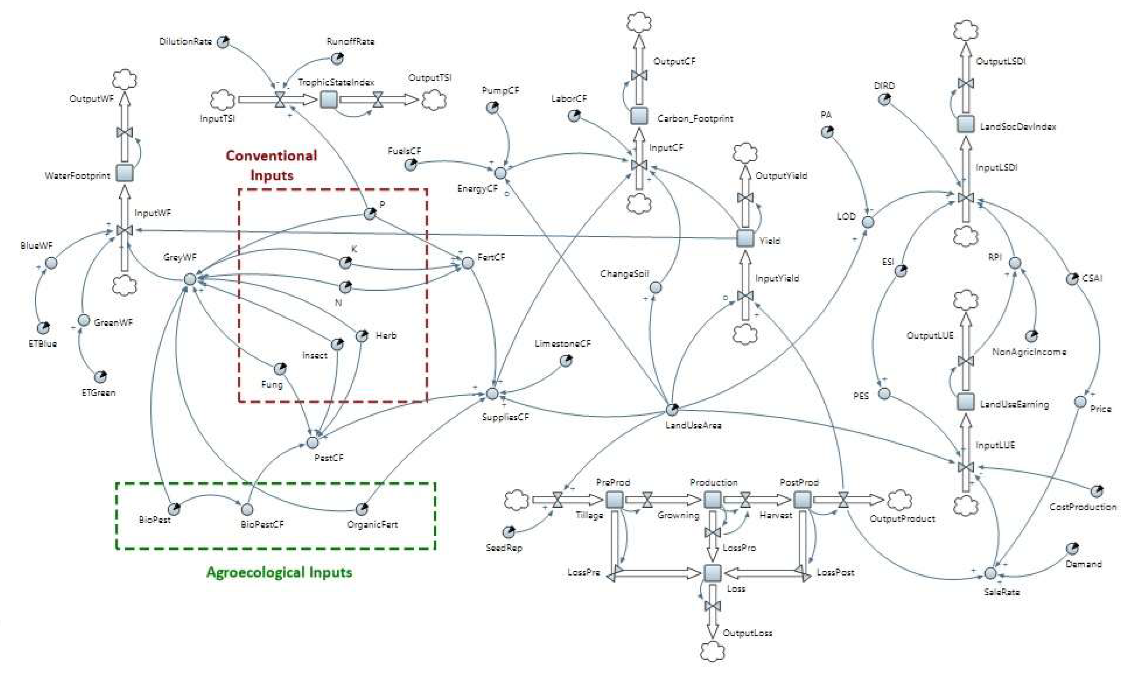
Figure 2. System Dynamics Model (SD-CoAg) for conventional and agroecological food production systems, Source: the authors. Legend: BioPest: biological pesticides; BioPestCF: biological pesticides carbon footprint; BlueWF: blue water footprint; CarbonFootprint: carbon footprint indicator stock; CSAI: community supported agriculture index; DIRD: demographic index of rural dependency; EnergyCF: energy carbon footprint; ESI: ecosystem service index; ETBlue: reference evapotranspiration; ETBGreen: crop evapotranspiration; FertCF: fertiliser carbon footprint; FuelsCF: fuels carbon footprint; Fung: fungicides; GreenWF: green water footprint; GreyWF: grey water footprint; Herb: herbicides; Insect: insecticides; InputCF: carbon footprint input flow; InputYield: yield input flow; InputLSDI: land social development index input flow; InputLUE: land use earnings input flow; InputTSI: trophic state index input flow; InputWF: water footprint input flow; K: potassium; LaborCF: carbon footprint labour; LandSocDevIndex: land social development index; LimestoneCF: limestone carbon footprint; LOD: land occupation degree; LossPre: loss of pre-production; LossPost: loss of post-production; LossPro: production loss; N: nitrogen; NonAgricIncome: non-agricultural income; OrganicFert: organic fertiliser; OutputCF: carbon footprint output flow; OutputLoss: total loss output flow; OutputProduct: product output flow; OutputYield: yield output flow; OutputLSDI: land social development index output flow; OutputLUE: land use earnings output flow; OutputTSI: trophic state index output flow; OutputWF: water footprint output flow; P: phosphorus; PA: property area; PestCF: pesticides carbon footprint; PreProd: pre-production; PostProd: post production; PumpCF: pump carbon footprint; PES: payment for environmental services; RPI: rural property income; SeedRep: seed replacement; SuppliesCF: supplies carbon footprint; Trophic State Index: trophic state index indicator stock; WaterFootprint: water footprint indicator stock; Yield: yield indicator stock.

The SD-CoAg model assesses synergies between society, the production system, and the environment via cause-and-effect analysis for predictive scenarios.

To illustrate the tool’s ability to respond to the aforementioned objective, researchers evaluated the causal links between commons stocks and certain parameters and/or dynamic variables (also considering the multiple impacts between different variables, such as those between product price and the CSAI, which shortens chains and allows producers to sell for a higher price), performing such simulations for agroecological (Ag) and conventional (Co) production methods. The components and input data that constitute the SDM-CoAg model are presented in Table 1.

Table 1. SDM-CoAg Model components and source, Source: the authors.

Parameter	Source
Limestone	Input data collected from pilot properties
Bio Pesticide	Bio-inputs used on family farms under “event” configuration, aiming at simulating the implementation of the ESI strategy (replacement by sources with greater efficiency)
Organic Fertilizer
Fungicide	Inputs used in Family properties under “event” configuration, aiming at simulating the implementation of ESI strategy (replacement of maximum concentrations for minimum)
Herbicide
Insect
Potassium/K
Nitrogen/N
Phosphorus/P
Cost Production	Collect secondary input data in São Paulo state database (https://www.cepea.esalq.usp.br/br/custos-de-producao.aspx, accessed on 3 March 2022)
Community-supported Agriculture Index (CSAI)	Simulated inputs under randomly configuration, due to lack of national historical data
Demand	Secondary collection in State databases, parameter under “seasonal event” configuration (https://ceagesp.gov.br/, accessed on 3 March 2022)
Dilution Rate	Secondary collection in State databases, parameter under “seasonal event” configuration for the Hydrographic Basin Baixo Tietê (https://sigrh.sp.gov.br/cbhat/apresentacao, accessed on 3 March 2022)
Ecosystem Services Index (ESI)	Parameter under “event” configuration aiming at simulating the implementation of ESI strategy for predictive scenarios
Demographic Index of Rural Dependency (DIRD)	Input data previously developed during the elaboration of the framework
Evapotranspiration Rate Blue (ETB)	Collect input in secondary databases ^[16]
Evapotranspiration Rate Green (ETG)	Collect input in secondary databases ^[16]
Fuels Carbon Footprint	Input data obtained via internationally validated tool used to obtain a CO2eq emission inventory ^[17]
Labour Carbon Footprint
Pump Carbon Footprint
Bio Pesticide Carbon Footprint
Energy Carbon Footprint
Fertilizer Carbon Footprint
Pesticide Carbon Footprint
Supplies Carbon Footprint
Land Use Area	Average area used by family producers (pilot plant)
Non-Agriculture Income	Given input, simulated a national minimum salary
Property Area (PA)	Average area of properties (pilot plant)
Runoff Rate	Collect input data in secondary databases ^[17], https://sigrh.sp.gov.br/cbhat/apresentacao, accessed on 3 March 2022)
Seed Reposition	Input data collected from pilot properties
Dynamic Variable	Source
Change Soil	Input data (equation) obtained via GHG Protocol (2010) tool ^[18]
Blue Water Footprint	Collect input data in secondary databases ^[17]
Green Water Footprint
Grey Water Footprint
Land Occupation Degree (LOD)	Average area of family properties (pilot plant)
Payment for Environment Services (PES)	Equation elaborated according to data obtained in secondary databases (Public Select Notion nº 006/2018, https://www.finatec.org.br/site/wp-content/uploads/2018/09/edital_PSA_006_2018.pdf, accessed on 3 March 2022)
Price	Equation elaborated according to data obtained in secondary databases (https://ceagesp.gov.br/, accessed on 3 March 2022; https://www.cepea.esalq.usp.br/br/custos-de-producao.aspx, accessed on 3 March 2022)
Sale Rate
Rural Property Income (RPI)	Equation previously developed during the elaboration of the framework (Figure 2)
Flux	Source
Growing	Input data referring to production on family properties (food production analysis)
Harvest
Output Product
Tillage
Input/Output Carbon Footprint	Some of CF considering on-site productivity (energy proxy)
Input/Output Land Social Development Index	Equation developed considering the average between the economic-social-environmental indicators
Input/Output Land Use Earnings	Equation developed considering the sale of local production
Input/Output TSI	Equation developed considering residual phosphorus and weather conditions ^[19]^[20]
Input/Output Water Footprint	Some of the WF considering on-site productivity—water proxy ^[17]
Input/Output Yield	Local productivity (food production analysis)
Loss Postproduction	Input data referring to family property losses
Loss Pre Production
Loss Production
Output Loss
Stock	Source
Carbon Footprint (CF)	Stocks of economic-social-environmental indicators developed from framework with data from pilot plant or according to secondary bases ^[17]^[18]^[19]^[20]
Land Social Development Index (LSDI)
Land Use Earning (LUE)
Trophic State Index (TSI)
Water Footprint (WF)
Loss	Inventories that represent local production and respective interferences, such as losses under productivity
Postproduction
Production
Yield

Behaviour curves of the cause–effect relationships mentioned were compared (Graphs T, U V, W, Z) with their respective benchmarks and divided into a ruler: pessimistic, neutral, or optimistic scenario, previously built based on the literature and technical protocols.

Some of the multiple cause–effect relationships between indicators and parameters or variables are displayed graphically (Figure 3, Figure 4, Figure 5, Figure 6 and Figure 7):

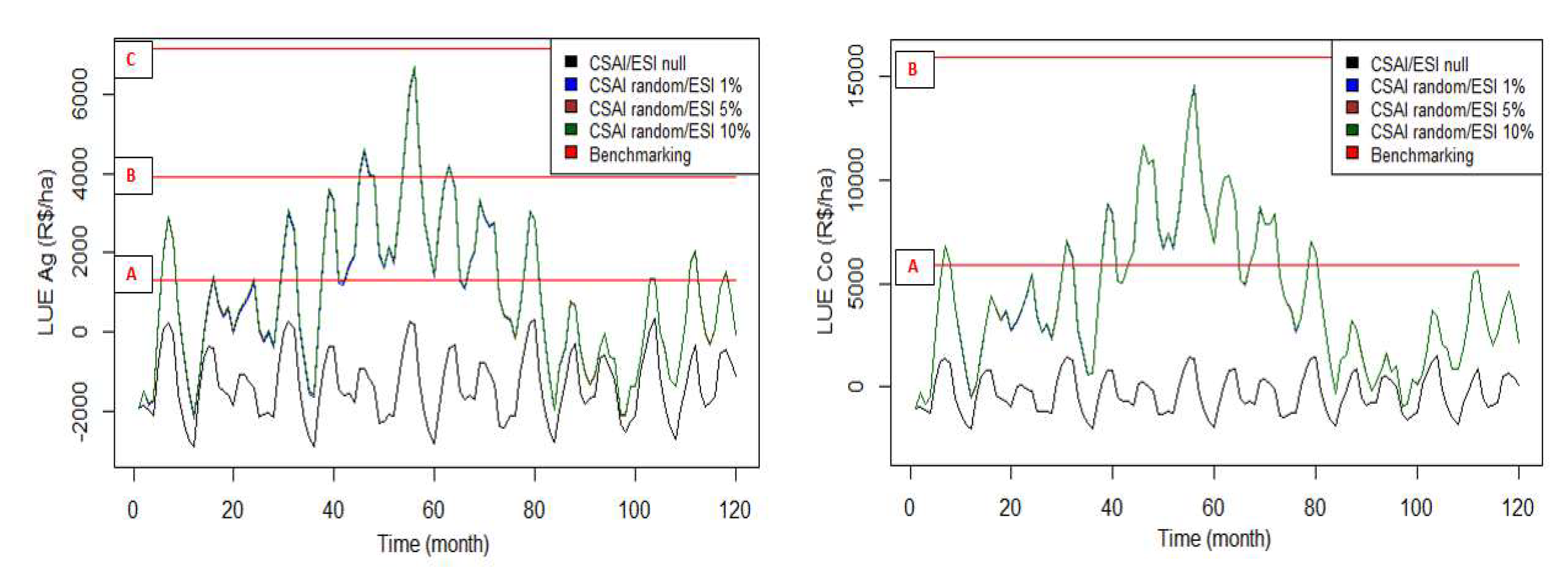
Figure 3. Land Use Earnings stock X Community Supported Agriculture Index (CSAI) and Payments for Environmental/Ecosystem Services (PES) parameters/dynamic variables, for agroecological (Ag) and conventional (Co) systems, Benchmarking—A: pessimistic level I; B: pessimistic level II; C: neutral, Source: the authors.

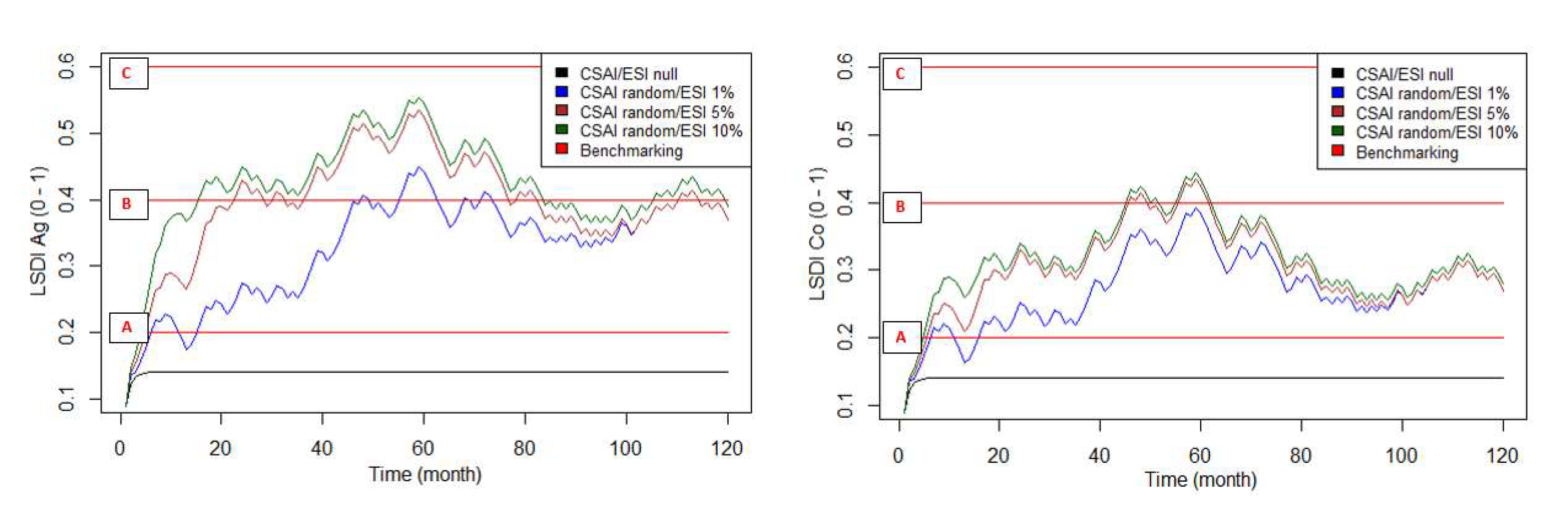
Figure 4. Land Use Social Development Index Stock X Community Supported Agriculture Index (CSAI) and Ecosystem Service Index (ESI) parameters, for agroecological (Ag) and conventional (Co) systems, Benchmarking—A: pessimistic level I; B: pessimistic level II; C: neutral, Source: the authors.

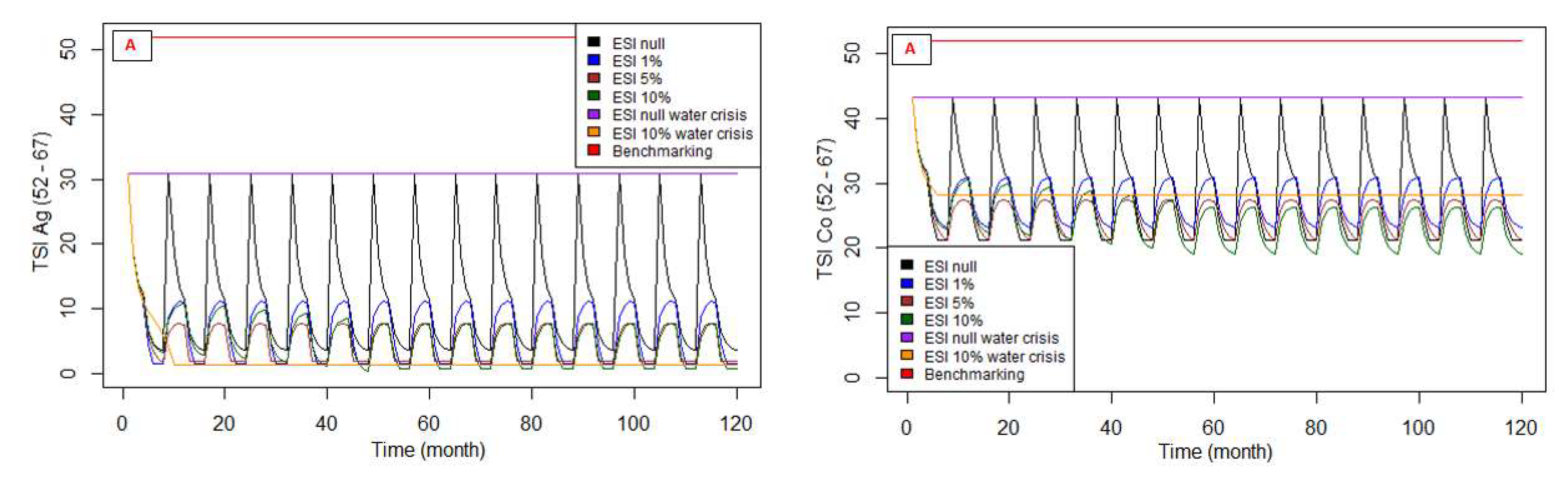
Figure 5. Tropic State Index (TSI) stock X Ecosystem Service Index (ESI) parameter for agroecological (Ag) and conventional (Co), in production units, Benchmarking—A: optimistic, Source: the authors.

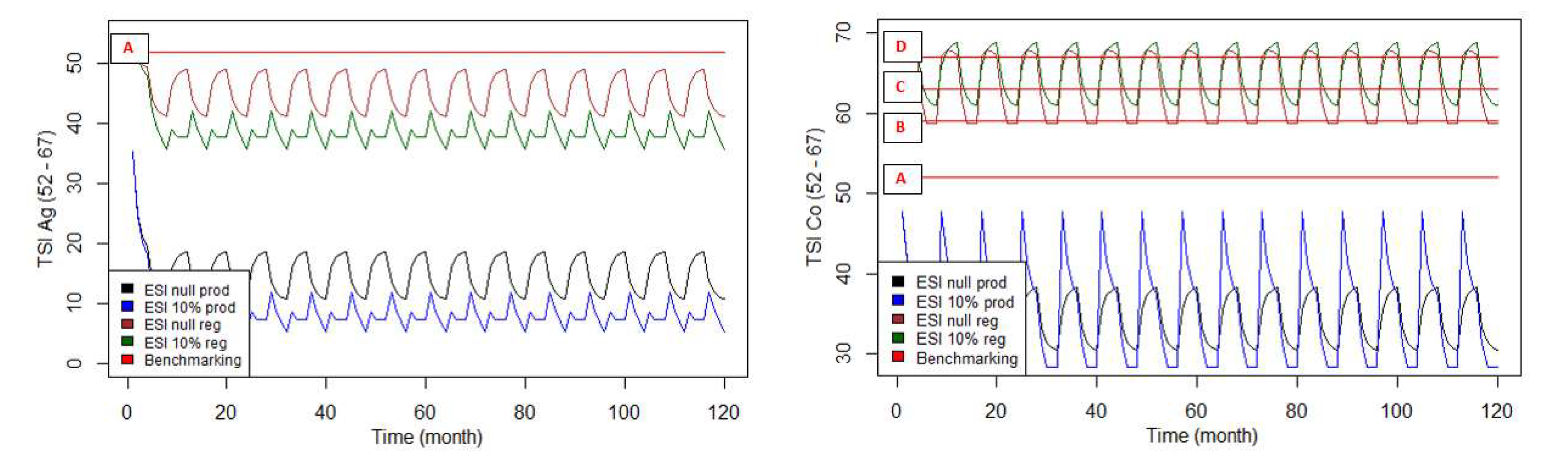
Figure 6. Tropic State Index (TSI) stock X Ecosystem Service Index (ESI) parameter for agroecological (Ag) and conventional (Co) systems, for an expanded area (1376 ha) in Southern São Paulo, Benchmarking—A: optimistic; B: optimistic; C: neutral; D: pessimistic, Source: the authors.

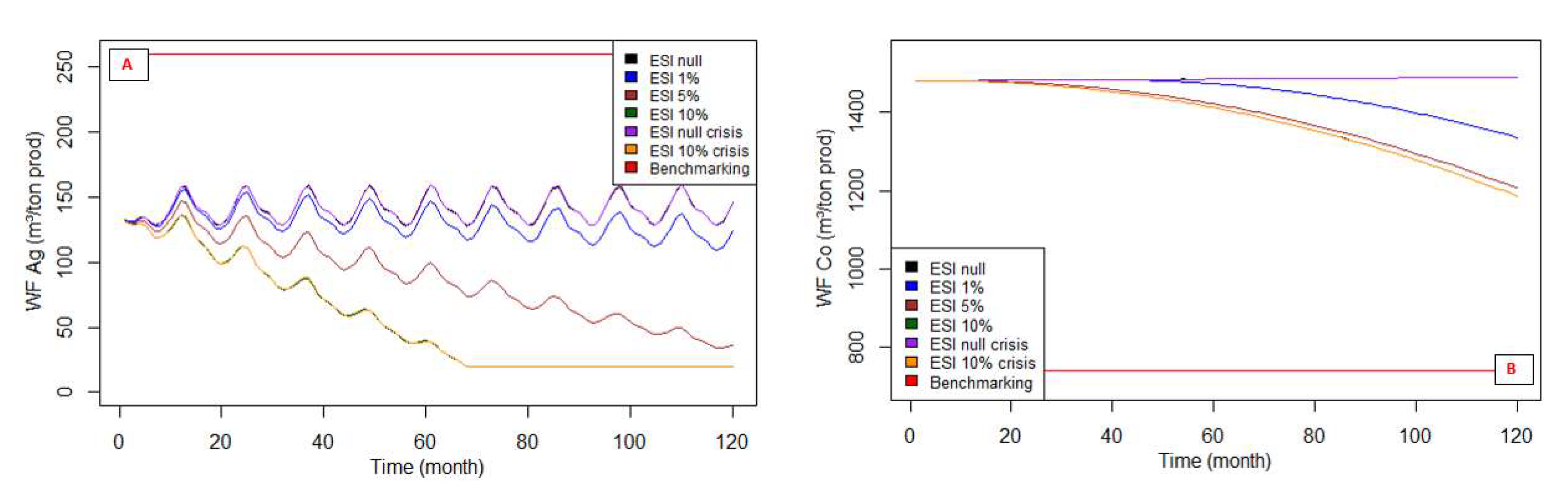
Figure 7. Water Footprint (WF) stock X Ecosystem Service Index (ESI) parameter, for agroecological (Ag) and conventional (Co) systems, Benchmarking—A: optimistic; B: pessimistic, Source: the authors.

Figure 3—Land Use Earnings stock (For the Land Use Earnings (LUE) and Land Social Development Index (LSDI) indicators, researchers considered four scenarios for a 10-year period—Scenario 1: null CSAI and ESI; Scenario 2: CSAI random and ESI with implementation of 1%/month, per hectare of the property; Scenario 3: CSAI random and ESI with implementation of 5%/month; Scenario 4: CSAI random and ESI with implementation of 10%/month) X Community Supported Agriculture Index (CSAI) and Payments for Environmental/Ecosystem Service (PES) parameters/dynamic variables;
Figure 4—Land Use Social Development Index Stock X Community Supported Agriculture Index (CSAI) and Ecosystem Service Index (ESI) parameters;
Figure 5—Tropic State Index (TSI) stock X Ecosystem Service Index (ESI) parameter (in this case, the strategy to reduce phosphorus not assimilated by the crops and leached via soil is substantiated by implementing Ecosystem Services, which aims to induce more sustainable practices, such as those that allow IST reduction);
Figure 6—Water Footprint (WF) stock X Ecosystem Service Index (ESI) parameter (in this case, the strategy to reduce nitrogen and chemicals and pesticides responsible for increasing the Grey Water Footprint (one of the components of total water footprint), is substantiated by implementing Ecosystem Services, which aims to induce more sustainable practices, such as those that allow WF reduction), and
Figure 7—Trophic State Index expanded to larger production area.

Researchers selected cause–effect relationships between stocks and parameters and variables for analysis because they represent highly relevant sustainability policies regarding current transition efforts, namely:

(a): Payments for Environmental Services (PES) (input data on ESI payments used as a benchmark, the Inter-American Development Bank (IBD) ruler, which was, in turn, used to implement the PES policy in the region under study at the border of the Atlantic Forest (Public Selection Notice PSA No. 006/2018), practiced by international development banks such as the World Bank, has the Ecosystem Service Index (ESI) payments indicator for land users who adopt sustainable commons practices, thus aligning their incentives with those of society as a whole ^[17] and generating ecosystem benefits.
(b): In the Community Supported Agriculture Index (CSAI) (programmed in random mode, via an automatic variation between 0 and 1, given the absence of historical CSAI data in countries for the practices under analysis), direct sales from producers to consumers relate to Land Use Earnings, since sales prices practiced without intermediaries can be higher.
(c): The Trophic State Index (TSI) (TSI was measured using the methodology of the environmental control and inspection agencies of the State of São Paulo, Brazil, as well as international protocols for this measurement, which interprets the phosphorus parameter as a measure of the eutrophication potential ^[18]^[19]. Measurement of the Water Footprint (WF) indicator for production systems considers the sum of the green, blue and grey water footprints representing the fraction of rainwater precipitated on the soil, the volume extracted from surface and/or underground springs, and the volume of water needed to dilute agricultural inputs, respectively ^[16]) ^[17]^[19]^[20], which measures the eutrophication process (since the eutrophication process is affected by climatic factors such as rainfall, which influences the flow of springs, researchers programmed the Dilution Rate parameter to simulate the seasonality of the region under study for scenarios 1 to 4), that is, it evaluates water quality, one of the FEW nexus’ direct stocks. Researchers evaluated the impacts of the parameters in productive units (1–4 ha) and in the pilot region under study (1376 ha, southern São Paulo).
(d): The Water Footprint (WF), a measure of water use in food production.

In the case of null CSAI and PES (scenario 1), researchers observed that for both systems, LUE has an essentially pessimistic profile; without the cited policies, LUE is at the limit of remuneration. In the Agroecological method, implementing the CSAI (all scenarios in which CSAI is positive) results in some improvement in LUE; the indicator goes from a pessimistic scale to neutral, emphasizing the importance of implementing CSAI strategies. On the other hand, in the conventional method, implementing the CSAI keeps LUE in a pessimistic benchmark band.

CSAI practice thus shows a differential vector impact for both production systems. Despite the positive influence of practices that result in PES, researchers see that the amount received monthly by producers has a marginal effect on the LUE indicator, not significantly influencing it for either production methods. This finding points to a review of the PES rates set in current PES grant notices.

This simulation clearly demonstrates the importance of CSAI and ESI policies for increasing land use social development (LSDI). Without implementing these practices (null CSAI and ESI), the LSDI profile is pessimistic for both systems (conventional and agroecological); that is, it is below the three benchmarks.

In scenarios where CSAI and ESI strategies are implemented, albeit asymmetrically, both modes of food production experience sustainability level gains.

Researchers observe an important evolution of this indicator for agroecological production, which goes from a pessimistic level to neutral in the 5% and 10% ESI scenarios, coming close to the optimistic profile. In conventional production, implementing these same strategies drives the indicator towards neutrality at times when the CSAI is highest for the 5% and 10% ESI scenarios.

However, it has a lower profile compared to the agroecological system, since the ESI can be implemented at a maximum of 0.5 (Public Selection Notice PSA No. 006/2018, from the São Paulo Forestry Institute, in joint policies with the Interamerican Development Bank, assigned an Environmental Services Index (ESI) for each of the modes of production, defined according to its potential to improve the region’s degree of sustainability. This index can reach a maximum of 0.5 in the conventional system and 1.0 for agroecology) in conventional systems, while it can reach 1.0 in agroecological, according to the guidelines of Notice No. 006/2018.

It is also relevant to observe that implementing 5% or 10% ESI does not significantly impact the levels of social and economic sustainability in both modes of production, suggesting a review of policies that establish gross values for payment for environmental services as a way to promote sustainability.

Figure 5 and Figure 6 below present the analysis of the relations between TSI and the ESI parameter for the two production methods; however, Figure 5 presents the dynamics modelling of 1ha properties, while Figure 6 analyses an expanded area of 1376 ha (referring to 344 properties of 1–4 ha on average, in southern São Paulo).

In the case of the agroecological system in any simulated scenario and area, individual property (1ha and 4ha) or expanded area (1376 ha), the result is TSI below the reference value 52 TSI (Trophic State Index, according to the methodology adopted by Brazilian national environmental regulatory agencies)—Oligotrophic; that is, agricultural activity in the region has a profile without undesirable interferences on water use.

For conventional production, in the case of a property (1 to 4ha), and considering both the absence and presence of TSI, all scenarios are sustainable, but come very close to the first benchmark (52 TSI—Oligotrophic).

When evaluating regional scenarios (1376 ha), however, researchers observe that the TSI profile moves between neutral and pessimistic benchmarks, even for the 10% ESI per month implementation scenario, across all properties. Neutral TSI (63 < TSI ≤ 59), called Eutrophic, shows reduced water transparency directly affected by human activities.

In the pessimistic benchmarking levels, TSI transits between the super eutrophic and hypereutrophic classifications, resulting in frequent undesirable changes in the quality of regional springs, caused by high concentration of organic matter and, at times (hypereutrophic), can present episodes of algae blooms and fish kills.

ESI implementation, which presupposes new practices to reduce the use of chemical and organic inputs in both systems, shows the importance of implementing ecosystem service strategies and techniques.

References

Dosi, G. Technological paradigms and technological trajectories: A suggested interpretation of the determinants and directions of technical change. Res. Policy 1982, 6, 147–162.
Levinthal, D.A. The slow pace of rapid technological change:gradualism and punctuation in technological change. Ind. Corp. Change 1998, 7, 217–247.
Nelson, R.R.; Winter, S.G. An Evolutionary Theory of Economic Change; Belknap Press: Cambridge, MA, USA, 1982.
Callon, M. Actor-network theory: The market test. In Actor Network Theory and After; Law, J., Hassard, J., Eds.; Blackwell Publishers: Oxford, UK, 1999; pp. 181–195.
Geels, F.W. Technological transitions as evolutionary recon-figuration processes: A multi-level perspective and a case-study. Res. Policy 2002, 31, 1257–1274.
Geels, F.W.; Elzen, B.; Green, K.; Elzen, B. General introdution: System innovation and transitions to sustainabilty. In System Innovation and the Transition to Sustainability: Theory, Evidence and Policy; Geels, F.W., Green, K., Eds.; Edward Elgar: Cheltenham, UK, 2004; Capítulo 1.
Ostrom, E.; James, W. Neither Markets Nor States: Linking Transformation Processes in Collective Action Arenas. In Perspectives on Public Choice: A Handbook; Dennis, C.M., Ed.; Cambridge University Press: Cambridge, UK, 1997; pp. 35–72.
Ostrom, E. Background on the institutional analysis and development framework. Policy Stud. J. 2011, 39, 7–27.
McGinnis, M.D.; Ostrom, E. Social-ecological system framework: Initial changes and continuing challenges. Ecol. Soc. 2014, 19, 30.
El Bilali, H. Transition heuristic frameworks in research on agro-food sustainability transitions. Environ. Dev. Sustain. 2018, 22, 1693–1728.
Bala, B.K.; Arshad, F.M.; Noh, K.M. System Dynamics Modelling and Simulation; Springer: Singapore, 2017.
Hajkowicz, S.; Negra, C.; Barnett, P.; Clark, M.; Harch, B.; Keating, B. Food price volatility and hunger alleviation: Can Cannes work? Agric. Food Secur. 2012, 1, 8.
Ahmad, S.; Tahar, R.M.; Muhammad Sukki, F.; Munir, A.B.; Rahim, R.A. Application of system dynamics approach in electricity sector modelling: A review. Renew. Sustain. Energy Rev. 2016, 56, 29–37.
Chhipi-Shrestha, G.; Hewage, K.; Sadiq, R. Water-Energy-Carbon Nexus Modelling for Urban Water Systems: System Dynamics Approach. J. Water Resour. Plann. Manag. 2017, 143, 04017016.
Forrester, J.W. Industrial Dynamics; MIT Press: Cambridge, MA, USA, 1961.
Forrester, J.W. Principles of System Dynamics; Productivity Press: Cambridge, MA, USA, 1968.
Hoekstra, A.Y.; Chapagain, A.K.; Aldaya, M.M.; Mekonnen, M.M. The Water Footprint Assessment Manual; E. Earthscan: Washington, DC, USA, 2011.
GHG. Programa Brasileiro GHG Protocol. 2010. Available online: https://www.ghgprotocolbrasil.com.br/ (accessed on 3 March 2021).
Lamparelli, M.C. Grau de Trofia em Corpos D’água do Estado de São Paulo: Avaliação dos Métodos de Monitoramento. Ph.D. Thesis, Instituto de Biociências, Universidade de São Paulo, São Paulo, Brazil, 2004.
CETESB (Companhia Ambiental do Estado de São Paulo). Índices de Qualidade das Águas—Apêndice D; CETESB: São Paulo, Brazil, 2017. Available online: https://cetesb.sp.gov.br/aguas-interiores/wp-content/uploads/sites/12/2017/11/Ap%C3%AAndice-D-%C3%8Dndices-de-Qualidade-das-%C3%81guas.pdf (accessed on 3 March 2021).

© Text is available under the terms and conditions of the Creative Commons Attribution (CC BY) license; additional terms may apply. By using this site, you agree to the Terms and Conditions and Privacy Policy.

Upload a video for this entry

Information

Subjects: Environmental Studies

Contributors MDPI registered users' name will be linked to their SciProfiles pages. To register with us, please refer to https://encyclopedia.pub/register :

Maria Ester Soares Dal Poz

Paulo Sergio de Arruda Ignacio

Anibal Tavares de Azevedo

Erika Cristina Francisco

Alessandro Luis Piolli

Gabriel Gheorghiu da Silva

Thais Pereira

View Times: 406

Entry Collection: Environmental Sciences

Update Date: 22 Jun 2022

Table of Contents

Video Upload Options

Confirm

1. Introduction

2. System Dynamics Modelling: The Backward-Looking Face of Janus

References