Submitted Successfully!
To reward your contribution, here is a gift for you: A free trial for our video production service.
Thank you for your contribution! You can also upload a video entry or images related to this topic.
Version Summary Created by Modification Content Size Created at Operation
1 -- 5628 2022-05-18 01:00:18 |
2 Reference format revised. -23 word(s) 5605 2022-05-18 04:30:42 |

Video Upload Options

Do you have a full video?

Confirm

Are you sure to Delete?
Cite
If you have any further questions, please contact Encyclopedia Editorial Office.
Bracamonte, J.; , .; Soares, J. Inverse Modeling in Cardiovascular Medicine. Encyclopedia. Available online: https://encyclopedia.pub/entry/23027 (accessed on 21 July 2024).
Bracamonte J,  , Soares J. Inverse Modeling in Cardiovascular Medicine. Encyclopedia. Available at: https://encyclopedia.pub/entry/23027. Accessed July 21, 2024.
Bracamonte, Johane, , Joao Soares. "Inverse Modeling in Cardiovascular Medicine" Encyclopedia, https://encyclopedia.pub/entry/23027 (accessed July 21, 2024).
Bracamonte, J., , ., & Soares, J. (2022, May 18). Inverse Modeling in Cardiovascular Medicine. In Encyclopedia. https://encyclopedia.pub/entry/23027
Bracamonte, Johane, et al. "Inverse Modeling in Cardiovascular Medicine." Encyclopedia. Web. 18 May, 2022.
Inverse Modeling in Cardiovascular Medicine
Edit

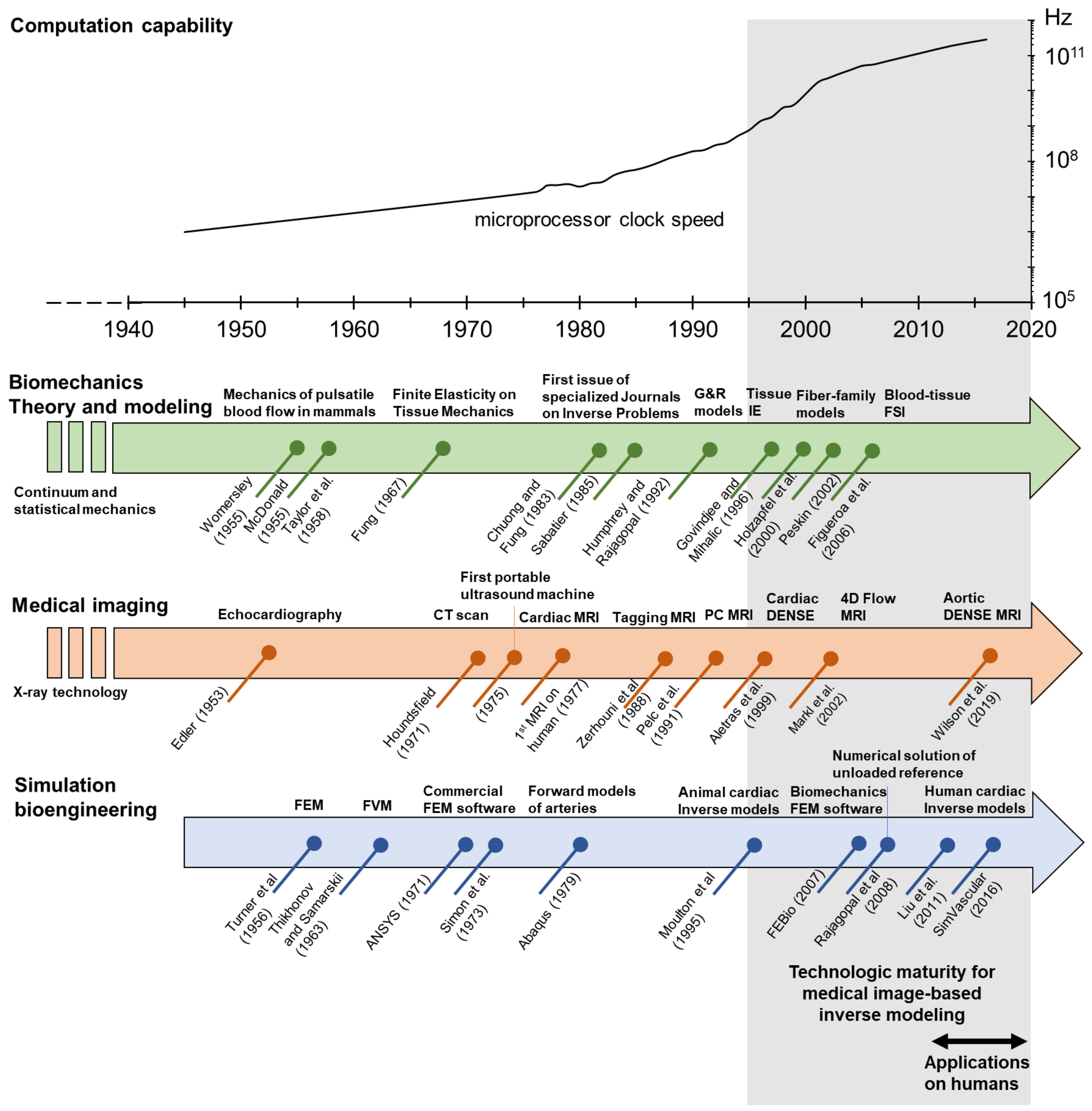
Inverse modeling approaches in cardiovascular medicine are a collection of methodologies that can provide non-invasive patient-specific estimations of tissue properties, mechanical loads, and other mechanics-based risk factors using medical imaging as inputs. Its incorporation into clinical practice has the potential to improve diagnosis and treatment planning with low associated risks and costs. Inverse method applications are multidisciplinary, requiring tailored solutions to the available clinical data, pathology of interest, and available computational resources. 

inverse models data assimilation cardiovascular imaging

1. Introduction

The primary role of numerical modeling in cardiovascular biomechanics has been to predict the performance of medical devices and to estimate physiological and mechanical cues acting on tissues, such as pressure and flow-driven stresses. Given the vast experimental evidence of mechanical factors producing effects on cellular differentiation, signaling, communication, and function [1][2][3][4][5], in silico experiments have explored the role of mechanical stimuli on normal and pathological tissue growth and remodeling [6]. From a clinical research standpoint, the development of patient-specific biomechanical models could provide more accurate and detailed data leading to a better understanding of the onset and progression of cardiovascular disease [7]. In addition, computational modeling has also been proposed as a supporting tool for medical practice on a patient-specific basis, which could provide non-invasive assessments of tissue properties, structure, and mechanical loads as physiologically meaningful risk stratification factors. Such patient-specific analyses have the potential to bring immense benefits to clinical practice by supporting diagnosis, treatment planning, and predictions of the outcome of surgical procedures with minimum associated costs and risk to the patients [8].
However, for biomechanical models to provide low-risk patient-specific solutions, personalized non-invasive clinical studies must be readily available to quantify regional cardiovascular function. Current medical imaging technology, namely echocardiography and magnetic resonance imaging (MRI), offers not only anatomical information but also high-resolution kinematics data of tissue motion and blood flow [9][10][11][12]. Kinematic-derived quantities, such as peak and average strain on the myocardium and aortic walls, have shown a good correlation with clinical risk markers [13]. Nevertheless, kinematic information alone cannot provide insights about mechanical forces, stresses, and tissue material properties, which are necessary for a full understanding of healthy and pathophysiological phenomena [14].
The inverse method, or data assimilation method, is an approach that allows solving classic mechanics problems “backwards”; that is, retrieving material properties and dynamic information (stress and forces) using measured kinematic information and loading boundary conditions as input [15]. Several research groups have coupled computational-mechanics tools with medical imaging technology to retrieve relevant biomechanical and hemodynamic markers from normal and pathological human tissues and organs [16], including diverse cardiovascular components [17]. Inverse modeling approaches have the potential to become a valuable tool for the non-invasive assessment of patient-specific cardiovascular health by providing quantitative physiological metrics that cannot be directly measured in vivo but may be derived entirely from clinical evaluations and the application of biomechanical principles.
Inverse modeling of biomechanical systems requires the confluence of state-of-the-art techniques from several disciplines including clinical care, medical imaging, simulation engineering, data analysis, and computer science (Figure 1).
/media/item_content/202205/6284544701880applsci-12-03954-g001.png
Figure 1. Timeline of microprocessor speed as a measure of computation capability, and relevant landmarks on the fields of biomechanics theory, medical imaging and simulation that make possible modern patient-specific image-based inverse modeling of the cardiovascular system. Acronyms: CT, computerized tomography; DENSE, displacement encoding with stimulated echoes; FEM, finite element method; FVM, finite volume method; IE, inverse elastostatics; FSI, fluid–structure interactions; PC, phase contrast; MRI, magnetic resonance imaging.
Inverse modeling analyses can also be applied to in vitro experimental setups. The main advantage of this approach is that input data is not limited by the available clinical tests, mechanical loads can be precisely controlled, and kinematics can be measured with high-resolution instruments. Furthermore, the target of the inverse method can be defined not only in terms of kinematic information but also in terms of controlled mechanical loads and stress measurements [18]. Moreover, the outputs of inverse modeling can be validated with controlled experimental parameters. Inverse analyses of in vitro setups have been applied to explanted animal and human tissue, and to engineered tissue constructs. Notably, inverse modeling has been applied to resolve mechanics at a cellular level.

2. Governing Principles of Biomechanics

2.1. Structural Mechanics of Cardiovascular Tissue

The study of soft biological tissues under the framework of finite elasticity was initiated by Y.C. Fung and others in the late 1960s, setting the basis of modern biomechanics [19][20]. As in classical solid mechanics, the mechanical analyses of cardiovascular tissues are usually performed with a Lagrangian formulation of the governing principles (Figure 2). Applied forces are imposed as boundary conditions. For blood vessels, these are prescribed as transmural pressure differences that often assume a traction-free condition on the adventitial surface. More recently, however, growing attention to the role of perivascular and pericardial support and tethering has promoted the inclusion of restrictions to the displacement of the outer surface of the heart and vasculature [14][21][22]. In addition, more complex formulations of cardiovascular tissue mechanics which departs from classical elastic solids have been proposed to account for complex microstructural compositions, the inclusion of pre-stress/strains, chemically activated muscular tone, and viscous energy dissipation.
Figure 2. Representation of the modeling process of structural mechanics of cardiovascular tissue and fluid mechanics of the blood flow with a continuum mechanics approach. Structural mechanics of cardiovascular tissue are usually analyzed with a Lagrangian formulation that follows the deformation of a given portion of the tissue. Blood flow mechanics is usually analyzed with an Eulerian formulation, that is, analyzing the mass and energy balances on a fixed volume of interest through which the fluid flows.
Cardiovascular tissues are comprised of multiple layers of cells and extracellular matrix (ECM) components. The ECM is a network of macromolecules that is continuously synthesized and degraded by active cells and functionally provides them with structural and biochemical support. Typically, collagen, elastin, and fibrillin are regarded as the main structural constituents responsible for the macroscopic mechanical behavior of cardiovascular tissues [23]. Healthy cardiovascular tissue retains residual stress even when unloaded (i.e., the tissue is pre-strained relative to a reference state of zero transmural pressure). Circumferential and axial pre-stress/strain in vascular conduits have been widely established by measuring how much these tissues recoil to an open configuration when excised and cut transversely and longitudinally to relieve the residual stress [24][25]. It has been hypothesized that pre-strain plays a relevant role in balancing higher stresses on the luminal surface of blood vessels and promoting a homogenized transmural stress distribution and homeostatic equilibrium of the vascular tissue [26]. Notably, residual strain is heterogeneous and has been shown to vary with patient age and health, likely as a consequence of heterogeneous growth and remodeling and/or damage.
Additionally, cardiovascular tissue is muscular in nature and actively contracts/distends. Thus, its mechanical behavior is affected by the activation of actin-myosin sliding filaments, which depends on ion-based chemical signaling and determines the muscular tone. In the myocardium, striated muscle activation is responsible for cardiac contraction. In large arteries, contraction of smooth muscle cells regulates downstream vascular resistance, blood flow, and propagation of the pressure-pulse wave along the vascular tree.
Of note, cardiovascular tissue also exhibits viscoelastic behavior, which has been established with stress relaxation, creep, and strain-rate experiments. It has been argued that viscous energy dissipation of healthy tissue, functioning at a regular physiological rate (~1 Hz), is negligible compared to stored strain energy [27]. Nevertheless, viscoelasticity may play a critical role under pathological conditions where the deformation rate is increased, such as in atrial fibrillation, or when dealing with highly dissipative structures such as lipid pools in atherosclerotic plaques [28][29]. Despite the relevance of viscoelastic properties to pathological conditions, standardized testing protocols have yet to be developed for the exploration of its relation to disease onset and progression [30]. Notably, if viscous dissipation and inertial effects are neglected, all temporal terms in the governing equations are canceled, rendering the problem a quasi-static process (which is the most common approach applied to vascular wall mechanics).

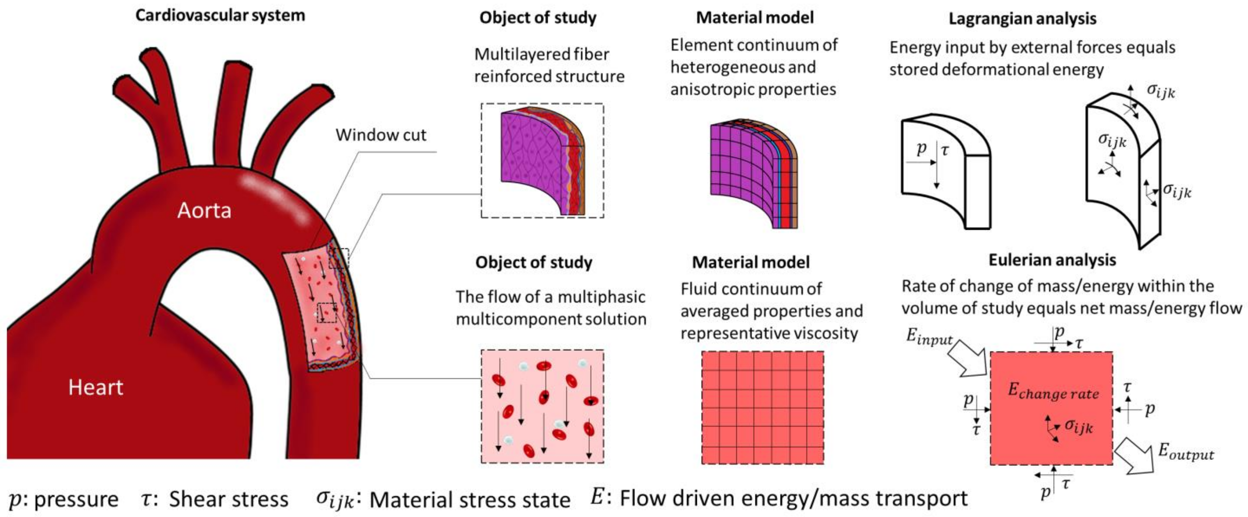
2.2. Fluid Mechanics of Blood Flow

For the study of fluids, it is more practical to implement an Eulerian formulation of the governing equations. This formulation is obtained by applying the Reynolds transport theorem to the equations for mass and momentum balance. Thus, this formulation solves the relation between flow driving forces, flow velocity, and deformation rates (Figure 2). A simplifying assumption applicable to biological systems is the incompressibility of the fluids, as most of them are either liquids or gases moving at subsonic velocities. Additionally, it is convenient to decompose the stress tensor into a spherical tensor representing the hydrostatic pressure and a deviatoric stress tensor. With this decomposition, constitutive equations can be designed to specifically relate the deviatoric stress components to the viscous dissipation of momentum.
Blood flow is generally assumed to be laminar throughout the circulatory system. The main arguments for this assumption are the pulsatile nature of the flow, the reduced dimensions of the vessels, and relatively low velocities, each contributing to the viscous effects overcoming the inertial forces and preventing turbulent random motion. However, it has been argued that transition to turbulent flows could be achieved locally in stenotic arteries. The use of a laminar model to study those cases could lead to an underestimation of wall shear stress, and stress oscillation [31][32]. Unlike most conventional engineering flows, blood flow is pulsatile and contained by compliant conduits of complex geometry. Since the 1950s, Womersley [33], McDonald [34], Taylor [35], Pedley [36], and others, developed analytical and experimental studies of pulsatile flow in mammals, identifying the most relevant parameters and features of this type of flow, thus setting the bases for modern hemodynamics.
Besides the intricacies of pulsatile flow in distensible conduits, the blood itself is a complex fluid. Blood consists of a suspension of cells in an aqueous solution of proteins and minerals called plasma. Plasma occupies approximately 55% of the blood volume, the rest being mainly occupied by red blood cells, white blood cells, and platelets. The rheological behavior of blood depends on how its constituents interact with each other and with the vessel walls, in consequence, this behavior is non-linear and highly dependent on the volumetric composition of blood, the flow conditions, and vessel dimensions. Modeling the complex interactions of blood constituents is a challenging statistical mechanics problem [37]. Some researchers have shown that cell aggregation and disaggregation are relevant to accurately describing blood rheology, especially in capillary flows where the cell size is comparable to the vessel diameter. Multiscale approaches have been successful in coupling the behavior of single cells as elastic entities with the transport equations of fluid flow, which are relevant for the study of clotting, aggregation, and platelet activation [38][39]. These approaches are computationally expensive, making them impractical for the study of large vessels.

2.3. Fluid-Structure Interactions (FSI)

Mechanics of the vascular wall and hemodynamics have been mostly studied as isolated problems; however, the function of the cardiovascular system is the result of complex interactions between blood, the actively contractile cardiac tissue, and the compliant vascular walls. The interaction of fluids and solids can conceptually be achieved by coupling the boundary conditions on the interface between the solid and the fluid, such that the field of displacements, velocities, and stresses are continuous and derivable at all points in a monolithic fully coupled approach. This, however, poses many implementation difficulties for complex 3D domains that can only be solved numerically. In addition, the typically large deformations of the cardiovascular walls cannot be handled by linearized methods used in conventional engineering applications.
The immersed boundary method, introduced by Peskin, was originally developed for the study of flow around heart valves and was rapidly adopted for many other applications [40]. In this approach, the Eulerian variables of fluid dynamics describing the surrounding flow are defined on a fixed computational grid, while the Lagrangian variables, accounting for the deformation of the tissue structures, are defined in a curvilinear computational grid that can be displaced with no conforming constraints in respect to the Eulerian grid. The moving solid boundary interacts with the fixed fluid domain by means of elastic body forces which are modulated by Dirac delta-like functions [41][42]. The fictitious domain method is a generalization of the immersed boundary method, which solves the coupling of the Lagrangian and Eulerian domains by the use of Lagrange multipliers instead of the concept of body forces [43]. This method is computationally less demanding as it does not require fitting the interface boundary at the cost of impaired accuracy near the interface.

3. Numerical Methods

3.1. Finite Volume Method

The finite volume method (FVM) is conceptually straightforward. The domain of study is discretized in a series of non-overlapping finite volumes, and the governing equations, usually expressed in Eulerian formulation, are converted into algebraic expressions by integrating them over each discrete volume. The balance equations are applied on a node located in the center of the finite volume, while the flux terms are calculated at its faces (Figure 3a). This allows first and second-order approximations of derivatives. The surface flow for a given shared face is set identical and in opposite direction for the adjacent discrete volumes, and equal to a boundary condition at the edge of the domain. By doing so, the balance equations are held at the whole domain and within each finite volume, which is one of the most attractive features of the FVM. Additionally, since the calculation of properties happens in the center of each volume, it is relatively easy to implement boundary conditions of a higher order [44]. Numerical implementation of this method is also straightforward in the case of structured meshes, becoming more complex for unstructured meshes due to the bookkeeping necessary for the calculations of interface flux balances.
Figure 3. Diagram of finite volume (FVM) and finite element methods (FEM) approximation principles. (a) In FVM, the domain is discretized in finite volumes, and balance equations are solved at the center of each volume. (b) In FEM, the domain is discretized in finite elements, and the variables distribution is assumed to follow a prescribed shape function within each finite element.

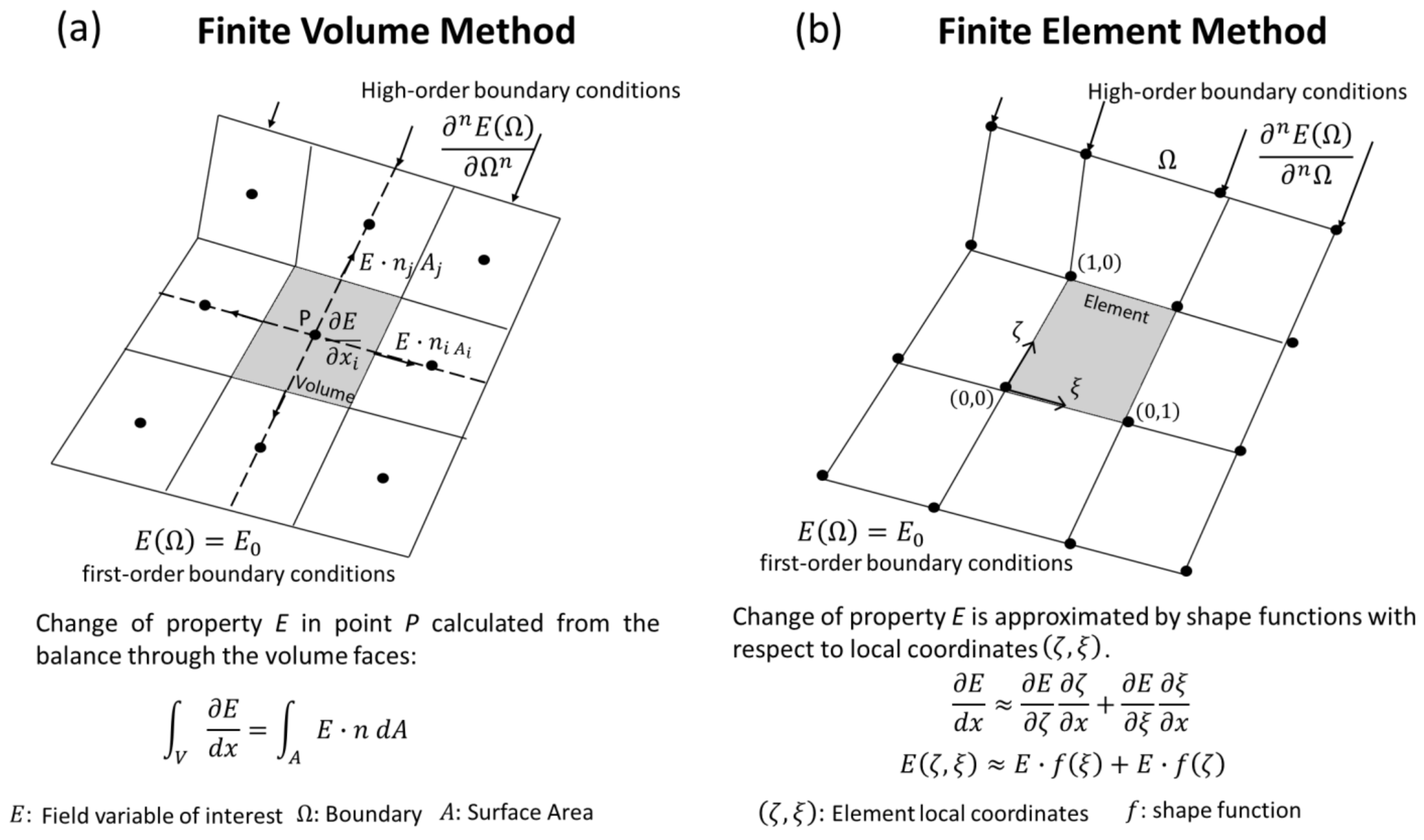
3.2. Finite Element Method (FEM)

The finite element method (FEM) consists of the discretization of the domain of study on simple geometrical elements (or finite elements), where the unknown fields are discretized as linear combinations of shape functions of any order, linear and quadratic being the most common. The shape functions are typically defined at each element depending on local and normalized coordinates (Figure 3b). The local governing equations for each element are then assembled and organized in a matricial system of algebraic equations. Finally, the solution is approximated by minimizing the weighted error associated with each element. Several weighting rules have been proposed, the Galerkin method and its variations being the most widely used [45]. By converging to the solution through the minimization of an error function and not through the exact solution of balance equations, FEM is said to be formulated in a “weak” form. However, the weak form is equivalent to the exact solution in the limit of refining the domain discretization. In fact, it has been widely shown that mesh-independent FEM solutions do not show any practical difference from the output of more conservative numerical methods such as FVM [46][47].

4. Inverse Problems

Modeling physical phenomena can be thought of as a mapping operation, where a set of inputs (B) is transformed into a set of outputs (E) by applying the model operator (M) such that M(B)=E. In the realm of physics, there must be a cause–effect relation between the inputs and outputs, and forward modeling consists of designing and applying a mapping function capable of producing outputs that closely follow experimental measurements (e), meaning that the difference Eshould be close to zero (Figure 4a) [48].
Figure 4. Data processing pipeline for patient-specific (a) forward problems and (b) direct inverse problems. Symbols, B: forward problem inputs, E: forward problem outputs, e: experimental data.
Conceptually, solving an inverse problem consists of using the measured effects to estimate the causes. That is, solving a problem of the type B=M1(e), which could be straightforward if M was a bijective function, with M and M1 being continuous and differentiable, and e was a continuous and smooth distribution (Figure 4b).

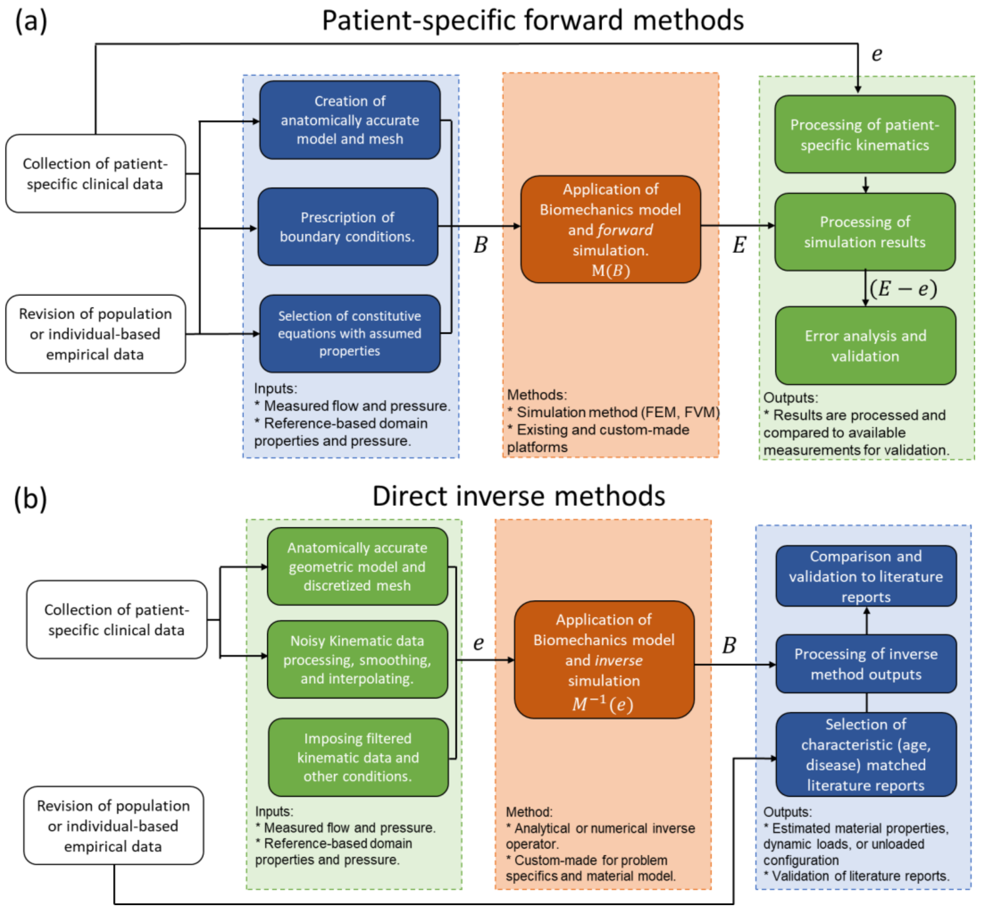
4.1. Direct Inverse Methods

The direct solution of inverse problems by the deduction of the inverse mapping function (M1) is only possible for oversimplified cases; however, specialized mathematics has been developed for the direct solution of some specific problems. In the case of finite elasticity, one relevant inverse problem is the retrieval of the mechanical properties of the domain of interest from the applied loads and measured displacement field. Several methods have been proposed to solve this problem directly, e.g., the reciprocity gap method which has been used to retrieve the distribution of elastic properties and to resolve the location of cracks in solid bodies from image-derived displacement fields. This method linearizes the inverse problem by assuming that the same elasticity tensor can resolve both the measured displacement field and a slightly perturbed version of it [15]. Another alternative for inverse elasticity is the application of the virtual work principle. This requires a complete description of the deformation field as a starting point, then the virtual work identity is defined by arbitrarily selecting a virtual field function. These functions can be tailored to specific constitutive equations to convert the virtual work identity into a set of algebraic equations from which the components of the elasticity tensor can be resolved [49][50].

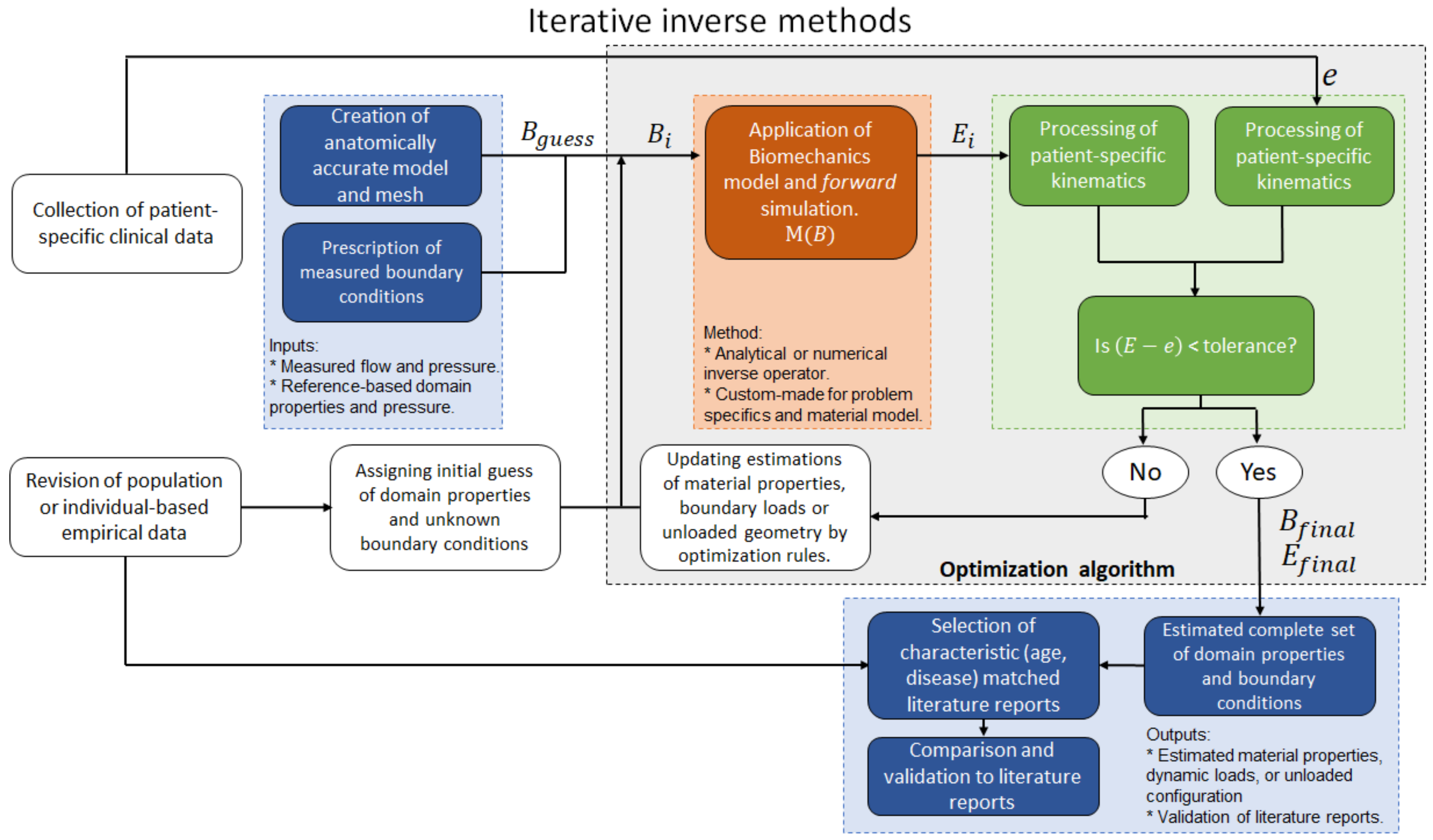
4.2. Iterative Inverse Methods

An alternative method for the solution of inverse problems is the iterative approach. This consists of optimization algorithms that iteratively solve the forward problem while varying the input parameters (B) until an error function defined as the difference between target experimental data (e) and the forward problem output (Eis minimized [51]. The advantages of this method are its easy generalization to any kind of inverse problem, its capability to operate on top of any existing solver for the forward problem, the existence of methods to reduce solution multiplicity, and its inherent capacity to handle scattered and noisy experimental data (Figure 5) [52]. All these advantages come with a detrimental increase in computational resource requirements, given by the repetitive solution of the forward problem. To reduce computational expense, some formulations have proposed the use of surrogate simpler models for the forward problem at the initial stages of the optimization process [53][54]. Some statistical tools based on Bayesian data analysis and inference have been implemented to improve the performance of iterative inverse methods for cases where the error distribution of the measured target is known or can be safely assumed [55].
Figure 5. Data processing pipeline for patient-specific iterative inverse methods. Symbols, B: forward problem inputs, E: forward problem outputs, e: experimental data.
The core concept of iterative inverse methods is the solution of an optimization problem that drives the solution into reproducing the target data with the smallest possible error. The definition of an optimization problem requires the selection of an appropriate target function to minimize, an optimization algorithm suited for the particular characteristics of the forward problem and optimization parameters, and the implementation of parameter constraints to point and restrict the convergence of the algorithm into desirable outputs. 

5. Medical Imaging-Based Kinematics

Early attempts to use medical imaging to assess the stiffness of blood vessels relied on the measurement of the luminal area change between diastolic and systolic configurations. This area change is used in several clinical risk markers, such as the β-index, that have shown a good correlation with the occurrence of certain cardiovascular pathologies such as atherosclerotic damage, hypertension, diabetes, and Marfan syndrome, as well as to tobacco exposure, obesity, aging, and other risk factors [56][57][58]. However, the predictive capabilities of these factors are inconsistent among different arterial locations and pathologies, most likely due to the oversimplification of the problem without any account of vascular mechanics [56].
In vivo medical imaging has evolved to provide not only anatomical geometric information but also detailed kinematics measurements. The accuracy and availability of these techniques are limited by image resolution, signal-to-noise ratio (SNR), the occurrence of artifacts, and practical obstacles related to testing costs and health hazards [59][60][61][62][63]

5.1. Ultrasound Technology (US)

Ultrasound (US) uses high frequency (2 to 15 MHz) acoustic waves to create real-time 2D in vivo images of tissues, organs, and blood pools using piezoelectric transducers. As in any wave, higher frequencies are associated with smaller wavelengths, higher penetration power, and improved image resolution [64][65]. Volume rendering from ultrasound images has led to three-dimensional, time-resolved ultrasound (4D US), and real-time imaging [66]. US is relatively inexpensive, portable, and safe, so it has become a customary tool in many clinical applications such as anesthesia, critical care, prenatal care, and pain management. Its application to cardiology, commonly known as echocardiography, was introduced in the 1950s, and currently is the more ubiquitous diagnostic tool to assess cardiovascular structure and function. With an approximate lateral resolution of 1 mm/pixel, this technique allows the estimation of heart chamber size, valve structure, identification of structural abnormalities such as seen in congenital heart defects (CHD), and determination of systolic and diastolic function (Figure 6c) [67]. Nevertheless, echocardiography presents some intrinsic limitations regarding accuracy and repeatability, particularly in patients with complex flow patterns related to congenital heart disease, aortic regurgitation, or dissection, in which case it is recommended to complement the study with other imaging techniques [68]. Intravascular ultrasound technology (IVUS) was developed following the principle that accuracy and resolution are improved as the transducer is closer to the tissue of interest. This technology involves placing a miniature ultrasound probe at the end of a catheter and then introducing the catheter into the vessel of interest in order to resolve the surrounding structures with greater detail than allowed by standard external US. This invasive technique is mostly used to study the conditions and progression of atherosclerosis in patients with coronary and carotid artery disease [69]. US technology can also provide blood flow and tissue kinematic information through the use of echo and vector Doppler and speckle tracking techniques.
Figure 6. Resolution comparison of left ventricular myocardium at diastole and systole with clinical grade (a) MRI, (b) CT (Reprinted/adapted with permission from Ref. [70], 2019, Korean Society of Echocardiography, open access), and (c) 2D ultrasound.

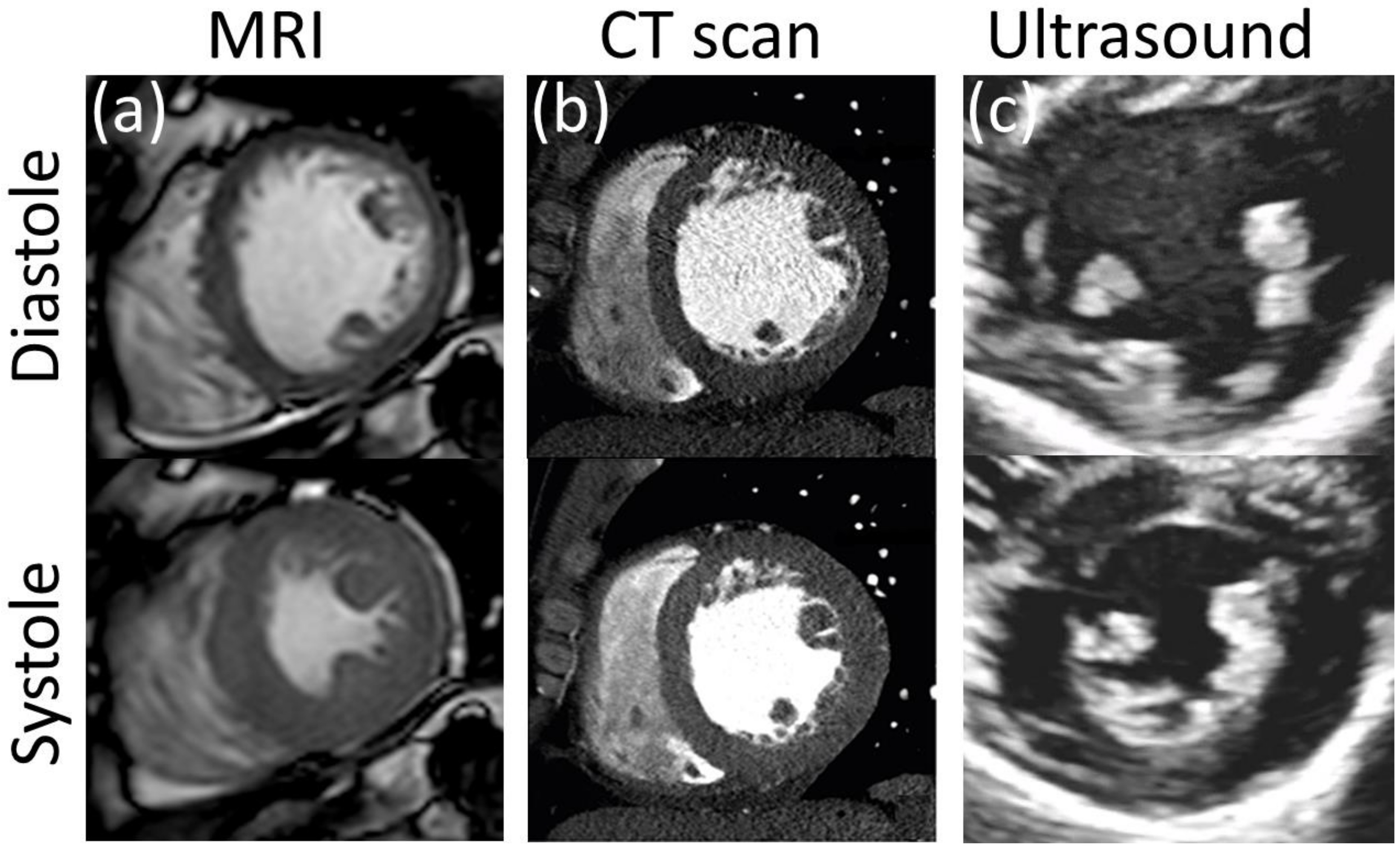
5.2. Magnetic Resonance Imaging (MRI)

Magnetic resonance imaging (MRI) offers superior quantitative utility compared to ultrasound as it offers high-resolution 2D and 3D visualization of the heart and major arteries referenced to a fixed coordinate system, providing greater accuracy for anatomic and volumetric assessment of heart chambers and wall thickness [71]. In addition, various MRI sequences have been specially designed to assess other valuable data such as fiber orientation, tissue displacement, and blood velocity [72][73].
The fundamental principle of this technology consists of the use of magnetic fields to align hydrogen protons in the body. After the magnetic field is interrupted, the protons return to a lower energy state by emitting radio signals that can be captured and utilized to create imaging data. For clinical applications, base magnetic fields with strengths ranging between 1.5 to 7 T are used to excite the protons to a base level. Then, a second time-varying radiofrequency magnetic field is used to induce changes in tissue magnetization. Tissues with different hydrogen-protons content will respond to the oscillating radiofrequency with different characteristic responses, which can be used to resolve various tissue components [74].

There are several options for MRI-based assessment of kinematics of both cardiovascular soft tissues and blood flow. Four prominent examples are: MRI tagging and displacement encoding with stimulated echoes (DENSE) for tissue displacement, and phase contrast and 4D flow MRI for blood flow quantification.

5.3. Computerized Tomography (CT)

CT consists of a mobile X-ray source that rotates around a focal point to produce scans from different angles. The result is a high-resolution stack of 2D images that can be time-resolved. The use of intravascular contrast agents is common for studies of the vascular system to improve the visibility of the blood vessels. CT scans can provide better resolution than all the other techniques described above with pixel sizes of about 0.5 mm (Figure 6b). There is no special feature to assess kinematics from CT scans, although its superior temporal and spatial resolution has been used to measure the dynamic change in cross-sectional area and shape of blood vessels during the cardiac cycle, from which homogenized values of circumferential strain for a given cross-section can be estimated. From there, kinematics can be inferred from tracking a given anatomical feature or making reasonable assumptions about rigid body rotation and torsion [11][75].
The use of ionizing radiation makes this technique potentially hazardous; thus risk-benefit of a CT study should be seriously considered. This limits its use in serial follow-up, particularly in pediatric patients, to avoid repetitive exposure to radiation [76]. However, it avoids the risk of unknown or contraindicated implanted metallic object/devices associated with MRI and is typically capable of much shorter scan times than MRI, making it ideal for trauma or other acute emergencies.

6. Applications to Cardiovascular Medicine

6.1. The Unloaded Reference Configuration in Cardiovascular Mechanics

Blood vessels, in particular those of the arterial tree, function under physiological pressure load at all times and are axially pre-stretched; thus, none of the patient-specific configurations resolved by in vivo imaging is truly a stress-free or zero-strain configuration [77]. It is well established that image-based estimations of material properties and stress distributions are sensitive to the selection of the reference configuration. Furthermore, image-based in vivo estimations of material properties assuming the diastolic configuration as a zero-strain stress-free reference lead to significant disagreements with experimental measurements made on excised tissue [78]. That means an adequate selection of the reference configuration is key for the accurate solution of inverse problems of cardiovascular tissue mechanics.
The solution of an unloaded configuration from the deformed geometry, mechanical loads, and material properties is a classical inverse problem with existing direct and iterative solutions [79]. In patient-specific analyses, however, the material properties are also unknown. Thus, the solution to this problem requires the specification of at least two deformed and loaded states as input data [80]. In the case of myocardium, it is often assumed that the transition from unloaded to diastolic configurations is purely passive [81]. Some iterative methods to determine the unloaded configuration are: backward displacement method [79] 237], the pull-back algorithm [238], and the shrink-and-fit algorithm [240]

6.2. The Heart

The relatively large thickness of cardiac tissue allowed the resolution of image-based kinematics even at the early stages of this technology. For this reason, along with the key role of the heart as the driving element of circulation, the heart was the first physiological system subject to patient-specific inverse analyses. Sermesant et al. and Aguado-Sierra et al. proposed comprehensive patient-specific models for cardiac function including the resolution of the unloaded configuration, bioelectrical activity, passive and active tissue properties, and hemodynamics [82][83]. These authors evaluated the possibility of solving such inverse problems with data acquired with medical imaging and electrocardiography and concluded that such comprehensive models easily became overparametrized, and computationally expensive to be solved by the available resources at the time. In consequence, most inverse models focus on only one or a few of their constituents instead of the whole heart.
The ventricular wall is a complex multilayered composite responsible for delivering the driving force to pump blood throughout the cardiovascular system. The myocardium is the functional layer of the ventricular wall, containing the myofibers responsible for the active contraction of the muscle and the structural collagen fibers that contribute to its bulk mechanical properties. An accurate understanding of myocardial mechanics is key for the diagnosis and treatment of diverse cardiac pathologies, and potentially, predicts and stratifies the risk of heart failure after infarct. Therefore, many inverse modeling studies have focused on the estimation of mechanical properties of healthy myocardium, and more interestingly, estimating the effects of ischemia, and quantifying the properties of infarcted cardiac tissue to yield a truly patient-specific risk assessment of cardiac failure [81][84][85][86][87][88][89][90][91][92].

6.3. Valves and Leaflets

Each one of the chambers of the heart is equipped with a discharge valve to ensure unidirectional blood flow, acting mostly passively to changes in transvalvular pressures. The atrioventricular valves are the mitral and tricuspid, for the left and right sides of the heart respectively. These valves typically define the basal plane and separate the atria from the ventricles. They are structurally supported by the papillary muscles and chordae tendineae to hold the valves closed during systole and avoid ventricle-to-atria backward flow. The pulmonary and aortic valves regulate blood flow from the ventricles to their homonym arteries and are not supported by any subvalvular apparatus. The main element of heart valves are fibrous structures called leaflets or cusps, that flap to allow or impede blood flow. In normal conditions, only the mitral valve has two leaflets while the other valves have three [93]. Heart valve disease is mostly related to regurgitation, stenosis, and atresia. The former consists of backflow due to deficient closing, stenosis is the hardening and thickening of the leaflets, preventing the valve to open properly and result in increased load in the heart, while the latter is a congenital disease where the heart valve is partially or completely absent. Heart valve malfunction can lead to several complications such as heart failure, blood clotting, stroke, and death. Heart valve disease is most common on the left side, as the aortic and mitral valves are loaded with larger pressures, and in consequence, they have received more attention from the medical and scientific community. However, attention to right heart valves has significantly grown in the last two decades along with the awareness of pulmonary artery diseases [94].

Leaflets are typically thin structures  showing complex displacement patterns, which renders them extremely challenging to resolve through in vivo imaging techniques. In vivo inverse modeling of ovine heart valves function has been achieved by the use of fluoroscopic markers implanted on the surface of mitral valve leaflets [95][96], a technique that cannot be pursued in human studies. More recently, Lee et al. applied ultrasound technology to assess the anatomy and displacement of the mitral valve of ovine animal models to explore the use of inverse modeling, and in vivo mechanical properties and stress distribution were successfully estimated [97][98]. Aggarwal et al. estimated the residual strain on human aortic valves by combining in vivo imaging with measurements on explanted tissues [99]. The authors collected in vivo transesophageal 3D echocardiographic images of the aortic valve from five open-heart transplant patients at three configurations: fully open, just-coapted, and fully loaded.

6.4. Arterial Wall

Changes in mechanical properties of arterial walls have been associated with the onset of multiple cardiovascular pathologies (e.g., atherosclerosis, dissection, stenosis) and remains an important predictor of cardiovascular morbidity and mortality in clinical practice. This motivated the development of early techniques for the non-invasive assessment of arterial stiffness through the evaluation of luminal area change and pulse wave velocity. These techniques, although useful, can only provide a gross estimation of material properties as they introduce many assumptions and simplifications related to homogeneity, perivascular support, and linearized behavior.
The image-based resolution of vascular tissue kinematics is technically challenging; the main reason being the relative thinness of vascular walls. For example, the ascending aorta has a typical thickness of about 2.5 mm, which decreases to about 1.5 mm at the abdominal aorta, and the pulmonary artery is only about 0.2 mm thick. These length scales are comparable to the highest resolutions available on imaging techniques, for which luminal area changes (either with or without contrast agents) remained the main input for early inverse analyses of arteries. However, recent developments in ultrasound speckle tracking and DENSE MRI techniques make available arterial wall displacement measurements on a meaningful number of pixels. 
Inverse modeling has been applied to estimate the mechanical properties of healthy arteries, aneurysms, and atherosclerotic plaques [100][101][102][103][104][105][106][107][108]. Additionally, inverse modeling has also been applied to estimate the effect of perivascular interactions on aortic mechanics [14][62][109]

6.5. Hemodynamics

In general, computational modeling of hemodynamics is more resource-consuming than tissue mechanics, as simulations need to account for transient effects and deal with the difficulties introduced by the non-linearities of convection and momentum dissipation. This makes the application of inverse modeling to hemodynamics a challenging task.
The use of simplified 0D (lumped) and 1D models can significantly reduce the computational cost. These simplified models have been used on a patient-specific basis and implemented onto inverse modeling approaches to provide useful systemic information about flow distribution, vascular resistance, and the systemic effect of drug treatments [110][111]. However, these approaches cannot exploit the detailed features offered by modern image-based kinematics as they only deal with 2D integrated or averaged metrics. Furthermore, despite all assumptions and simplifications, inverse approaches to lumped and 1D models are still prone to solution multiplicity [112].
To deal with the computational expense of the forward problem on inverse hemodynamics, Lassila et al. proposed a method for parametrizing the Navier–Stokes equations and patient-specific geometries to reduce the basis of the partial differential equations. The parameterized model is iteratively solved until the algorithm is close to the final solution. At this point, the inverse method then switches to the solution of the full-forward problem using FVM. This method was tested using deterministic and Bayesian optimization algorithms showing promising results in the solution of test cases involving rigid-wall and FSI simulations [53].

Zambrano et al. proposed an iterative inverse method for the study of the pulmonary artery [113]. Intravascular pressure measurements, PC MRI at the main branches of the pulmonary artery, and cine MRI were collected from a pulmonary hypertensive adult patient and a healthy volunteer with no reported cardiovascular disease. A 3D model from the main pulmonary artery (MPA) down to the 4th branch generation was built from MRI images at the end-diastole configuration, which was considered stress-free. MRI-derived diameter changes were calculated at the main pulmonary artery and coupled to pressure measurements.The proposed model was able to reproduce the expected increase in arterial stiffness and vascular flow resistance in the hypertensive patient. In a follow-up study, the methodology was applied to a cohort of six individuals with pulmonary artery hypertension and five healthy volunteers [114].

References

  1. Kakisis, J.D.; Liapis, C.D.; Sumpio, B.E. Effects of Cyclic Strain on Vascular Cells. Endothelium 2004, 11, 17–28.
  2. Chang, H.-I.; Wang, Y. Cell response to surface and architecture of tissue engineering scaffolds. In Regenerative Medicine and Tissue Engineering—Cells and Biomaterials; Eberli, D., Ed.; InTech Open Access Publisher: Rijeka, Croatia, 2011.
  3. Butler, D.L.; Goldstein, S.A.; Guilak, F. Functional Tissue Engineering: The Role of Biomechanics. J. Biomech. Eng. 2000, 122, 570–575.
  4. Tang, B.T.; Pickard, S.S.; Chan, F.P.; Tsao, P.S.; Taylor, C.A.; Feinstein, J.A. Wall Shear Stress is Decreased in the Pulmonary Arteries of Patients with Pulmonary Arterial Hypertension: An Image-Based, Computational Fluid Dynamics Study. Pulm. Circ. 2012, 2, 470–476.
  5. Pourmodheji, R.; Jiang, Z.; Tossas-Betancourt, C.; Figueroa, C.A.; Baek, S.; Lee, L.-C. Inverse modeling framework for characterizing patient-specific microstructural changes in the pulmonary arteries. J. Mech. Behav. Biomed. Mater. 2021, 119, 104448.
  6. Watton, P.N.; Hill, N.A. Evolving mechanical properties of a model of abdominal aortic aneurysm. Biomech. Model. Mechanobiol. 2009, 8, 25–42.
  7. Neal, M.L.; Kerckhoffs, R. Current progress in patient-specific modeling. Brief. Bioinform. 2010, 11, 111–126.
  8. Marsden, A.; Esmaily-Moghadam, M. Multiscale Modeling of Cardiovascular Flows for Clinical Decision Support. Appl. Mech. Rev. 2015, 67, 030804.
  9. Itatani, K.; Miyazaki, S.; Furusawa, T.; Numata, S.; Yamazaki, S.; Morimoto, K.; Makino, R.; Morichi, H.; Nishino, T.; Yaku, H. New imaging tools in cardiovascular medicine: Computational fluid dynamics and 4D flow MRI. Gen. Thorac. Cardiovasc. Surg. 2017, 65, 611–621.
  10. Wilson, J.S.; Zhong, X.; Hair, J.B.; Taylor, W.R.; Oshinski, J.N. In Vivo Quantification of Regional Circumferential Green Strain in the Thoracic and Abdominal Aorta by Two-Dimensional Spiral Cine DENSE MRI. J. Biomech. Eng. 2019, 141, 0609011–06090111.
  11. Kong, F.; Shadden, S.C. Automating Model Generation for Image-Based Cardiac Flow Simulation. J. Biomech. Eng. 2020, 142, 1110111–11101113.
  12. Markl, M.; Schnell, S.; Barker, A. 4D Flow Imaging: Current Status to Future Clinical Applications. Curr. Cardiol. Rep. 2014, 16, 481.
  13. Wilson, J.S.; Taylor, W.R.; Oshinski, J. Assessment of the regional distribution of normalized circumferential strain in the thoracic and abdominal aorta using DENSE cardiovascular magnetic resonance. J. Cardiovasc. Magn. Reson. 2019, 21, 59.
  14. Bracamonte, J.H.; Wilson, J.S.; Soares, J.S. Assessing Patient-Specific Mechanical Properties of Aortic Wall and Peri-Aortic Structures from In Vivo DENSE Magnetic Resonance Imaging Using an Inverse Finite Element Method and Elastic Foundation Boundary Conditions. J. Biomech. Eng. 2020, 142, 1210111–12101113.
  15. Bonnet, M.; Constantinescu, A. Inverse problems in elasticity. Inverse Probl. 2005, 21, R1–R50.
  16. Wang, W.; Wang, D.; Falisse, A.; Severijns, P.; Overbergh, T.; Moke, L.; Scheys, L.; De Groote, F.; Jonkers, I. A Dynamic Optimization Approach for Solving Spine Kinematics While Calibrating Subject-Specific Mechanical Properties. Ann. Biomed. Eng. 2021, 49, 2311–2322.
  17. Zhang, Y.; Wang, V.Y.; Morgan, A.E.; Kim, J.; Ge, L.; Guccione, J.M.; Weinsaft, J.W.; Ratcliffe, M.B. A Novel MRI-Based Finite Element Modeling Method for Calculation of Myocardial Ischemia Effect in Patients with Functional Mitral Regurgitation. Front. Physiol. 2020, 11, 158.
  18. Avazmohammadi, R.; Li, D.S.; Leahy, T.; Shih, E.; Soares, J.S.; Gorman, J.H.; Gorman, R.C.; Sacks, M.S. An integrated inverse model-experimental approach to determine soft tissue three-dimensional constitutive parameters: Application to post-infarcted myocardium. Biomech. Model. Mechanobiol. 2018, 17, 31–53.
  19. Fung, Y.C. Elasticity of soft tissues in simple elongation. Am. J. Physiol. Content 1967, 213, 1532–1544.
  20. Chuong, C.J.; Fung, Y.C. Three-Dimensional Stress Distribution in Arteries. J. Biomech. Eng. 1983, 105, 268–274.
  21. Pfaller, M.R.; Hörmann, J.M.; Weigl, M.; Nagler, A.; Chabiniok, R.; Bertoglio, C.; Wall, W.A. The importance of the pericardium for cardiac biomechanics: From physiology to computational modeling. Biomech. Model. Mechanobiol. 2019, 18, 503–529.
  22. Liu, Y.; Dang, C.; Garcia, M.; Gregersen, H.; Kassab, G.S. Surrounding tissues affect the passive mechanics of the vessel wall: Theory and experiment. Am. J. Physiol. Circ. Physiol. 2007, 293, 3290–3300.
  23. Humphrey, J.D. Mechanics of the Arterial Wall: Review and Directions. Crit. Rev. Biomed. Eng. 1995, 23, 1–162.
  24. Sokolis, D.P.; Savva, G.D.; Papadodima, S.A.; Kourkoulis, S.K. Regional distribution of circumferential residual strains in the human aorta according to age and gender. J. Mech. Behav. Biomed. Mater. 2017, 67, 87–100.
  25. Sokolis, D.P.; Bompas, A.; Papadodima, S.A.; Kourkoulis, S.K. Variation of Axial Residual Strains along the Course and Circumference of Human Aorta Considering Age and Gender. J. Biomech. Eng. 2020, 142, 0210031–02100313.
  26. Cardamone, L.; Valentín, A.; Eberth, J.F.; Humphrey, J.D. Origin of axial prestretch and residual stress in arteries. Biomech. Model. Mechanobiol. 2009, 8, 431–446.
  27. Holzapfel, G.; Gasser, T.; Stadler, M. A structural model for the viscoelastic behavior of arterial walls: Continuum formulation and finite element analysis. Eur. J. Mech. A Solids 2002, 21, 441–463.
  28. Humphrey, J.D.; Na, S. Elastodynamics and Arterial Wall Stress. Ann. Biomed. Eng. 2002, 30, 509–523.
  29. Akyildiz, A.C.; Speelman, L.; Gijsen, F.J.H. Mechanical properties of human atherosclerotic intima tissue. J. Biomech. 2014, 47, 773–783.
  30. Wang, Z.; Golob, M.J.; Chesler, N.C. Viscoelastic Properties of Cardiovascular Tissues. Viscoelast. Viscoplast. Mater. 2016, 2, 64.
  31. Barker, A.J.; van Ooij, P.; Bandi, K.; Garcia, J.; Albaghdadi, M.; McCarthy, P.; Bonow, R.O.; Carr, J.; Collins, J.; Malaisrie, S.C.; et al. Viscous energy loss in the presence of abnormal aortic flow. Magn. Reson. Med. 2014, 72, 620–628.
  32. Mahalingam, A.; Gawandalkar, U.U.; Kini, G.; Buradi, A.; Araki, T.; Ikeda, N.; Nicolaides, A.; Laird, J.R.; Saba, L.; Suri, J.S. Numerical analysis of the effect of turbulence transition on the hemodynamic parameters in human coronary arteries. Cardiovasc. Diagn. Ther. 2016, 6, 208–220.
  33. Womersley, J.R. Method for the calculation of velocity, rate of flow and viscous drag in arteries when the pressure gradient is known. J. Physiol. 1955, 127, 553–563.
  34. McDonald, D.A. The relation of pulsatile pressure to flow in arteries. J. Physiol. 1955, 127, 533–552.
  35. Taylor, M.G. The Discrepancy between Steady- and Oscillatory-Flow Calibration of Flowmeters of the ‘Bristle’and ‘Pendulum’ Types: A Theoretical Study. Phys. Med. Biol. 1958, 2, 324–337.
  36. Pedley, T.J.; Schroter, R.C.; Sudlow, M.F. Pressure flow relations in branched tubes. J. Physiol. 1969, 204, 114. Available online: https://europepmc.org/article/med/5824621 (accessed on 29 November 2021).
  37. Williams, M.C.; Rosenblatt, J.S.; Soane, D.S. Theory of Blood Rheology Based on a Statistical Mechanics Treatment of Rouleaux, and Comparisons with Data. Int. J. Polym. Mater. Polym. Biomater. 1993, 21, 57–63.
  38. Soares, J.S.; Gao, C.; Alemu, Y.; Slepian, M.; Bluestein, D. Simulation of platelets suspension flowing through a stenosis model using a dissipative particle dynamics approach. Ann. Biomed. Eng. 2013, 41, 2318–2333.
  39. Fedosov, D.A.; Noguchi, H.; Gompper, G. Multiscale modeling of blood flow: From single cells to blood rheology. Biomech. Model. Mechanobiol. 2013, 132, 239–258.
  40. Peskin, C.S. The immersed boundary method. Acta Numer. 2002, 11, 479–517.
  41. Flamini, V.; DeAnda, A.; Griffith, B.E. Immersed boundary-finite element model of fluid–structure interaction in the aortic root. Theor. Comput. Fluid Dyn. 2015, 30, 139–164.
  42. Yang, X.; Zhang, X.; Li, Z.; He, G.W. A smoothing technique for discrete delta functions with application to immersed boundary method in moving boundary simulations. J. Comput. Phys. 2009, 228, 7821–7836.
  43. van Loon, R.; Anderson, P.D.; van de Vosse, F.; Sherwin, S. Comparison of various fluid–structure interaction methods for deformable bodies. Comput. Struct. 2007, 85, 833–843.
  44. Moukalled, F.D.F.; Mangani, L. The Finite Volume Method in Computational Fluid Dynamics; Springer: New York, NY, USA, 2015.
  45. Mackerle, J. Finite element modelling and simulations in cardiovascular mechanics and cardiology: A bibliography 1993–2004. Comput. Methods Biomech. Biomed. Eng. 2005, 8, 59–81.
  46. Fallah, N.A.; Bailey, C.; Cross, M.; Taylor, G. Comparison of finite element and finite volume methods application in geometrically nonlinear stress analysis. Appl. Math. Model. 2000, 24, 439–455.
  47. Jeong, W.; Seong, J. Comparison of effects on technical variances of computational fluid dynamics (CFD) software based on finite element and finite volume methods. Int. J. Mech. Sci. 2014, 78, 19–26.
  48. Sabatier, P.C. Inverse Problems—An introduction. Inverse Probl. 1985, 1, 302.
  49. Grédiac, M.; Toussaint, E.; Pierron, F. Special virtual fields for the direct determination of material parameters with the virtual fields method. 2—Application to in-plane properties. Int. J. Solids Struct. 2002, 39, 2707–2730.
  50. Grediac, M.; Toussaint, E.; Pierron, F. Special virtual fields for the direct determination of material parameters with the virtual fields method. 1—Principle and definition. Int. J. Solids Struct. 2002, 39, 2691–2705.
  51. Tessler, A.; Spangler, J.L. A least-squares variational method for full-field reconstruction of elastic deformations in shear-deformable plates and shells. Comput. Methods Appl. Mech. Eng. 2005, 194, 327–339.
  52. Beck, J.V.; A Woodbury, K.A. Inverse problems and parameter estimation: Integration of measurements and analysis. Meas. Sci. Technol. 1998, 9, 839–847.
  53. Lassila, T.; Manzoni, A.; Quarteroni, A.; Rozza, G. A reduced computational and geometrical framework for inverse problems in hemodynamics. Int. J. Numer. Methods Biomed. Eng. 2013, 29, 741–776.
  54. Liu, M.; Liang, L.; Sun, W. A new inverse method for estimation of in vivo mechanical properties of the aortic wall. J. Mech. Behav. Biomed. Mater. 2017, 72, 148–158.
  55. Cotter, S.L.; Dashti, M.; Robinson, J.C.; Stuart, A.M. Bayesian inverse problems for functions and applications to fluid mechanics. Inverse Probl. 2009, 25, 115008.
  56. Wohlfahrt, P.; Krajčoviechová, A.; Seidlerová, J.; Mayer, O.; Bruthans, J.; Filipovský, J.; Laurent, S.; Cífková, R. Arterial stiffness parameters: How do they differ? Atherosclerosis 2013, 231, 359–364.
  57. Vitarelli, A.; Conde, Y.; Cimino, E.; D’Angeli, I.; D’Orazio, S.; Stellato, S.; Padella, V.; Caranci, F. Aortic Wall Mechanics in the Marfan Syndrome Assessed by Transesophageal Tissue Doppler Echocardiography. Am. J. Cardiol. 2006, 97, 571–577.
  58. Mack, W.J.; Islam, T.; Lee, Z.; Selzer, R.H.; Hodis, H.N. Environmental tobacco smoke and carotid arterial stiffness. Prev. Med. 2003, 37, 148–154.
  59. Töger, J.; Zahr, M.J.; Aristokleous, N.; Bloch, K.M.; Carlsson, M.; Persson, P.-O. Blood flow imaging by optimal matching of computational fluid dynamics to 4D-flow data. Magn. Reson. Med. 2020, 84, 2231–2245.
  60. Hess, A.T.; Bissell, M.M.; Ntusi, N.A.B.; Lewis, A.J.M.; Tunnicliffe, E.M.; Greiser, A.; Stalder, A.F.; Francis, J.M.; Myerson, S.G.; Neubauer, S.; et al. Aortic 4D flow: Quantification of signal-to-noise ratio as a function of field strength and contrast enhancement for 1.5 T, 3 T, and 7 T. Magn. Reson. Med. 2015, 73, 1864–1871.
  61. Aletras, A.H.; Ding, S.; Balaban, R.S.; Wen, H. DENSE: Displacement Encoding with Stimulated Echoes in Cardiac Functional MRI. J. Magn. Reson. 1999, 137, 247–252.
  62. Bracamonte, J.H.; Wilson, J.S.; Soares, J.S. Quantification of the heterogeneous effect of static and dynamic perivascular struc-tures on patient-specific local aortic wall mechanics using inverse finite element modeling and DENSE MRI. J. Biomech. 2009, 11, 123.
  63. Busch, J.; Giese, D.; Kozerke, S. Image-based background phase error correction in 4D flow MRI revisited. J. Magn. Reson. Imaging 2017, 46, 1516–1525.
  64. Ng, A.; Swanevelder, J. Resolution in ultrasound imaging. Contin. Educ. Anaesth. Crit. Care Pain 2011, 11, 186–192.
  65. Sassaroli, E.; Crake, C.; Scorza, A.; Kim, D.; Park, M. Image quality evaluation of ultrasound imaging systems: Advanced B-modes. J. Appl. Clin. Med. Phys. 2019, 20, 115–124.
  66. Linte, C.A.; Moore, J.; Wiles, A.D.; Wedlake, C.; Peters, T.M. Virtual reality-enhanced ultrasound guidance: A novel technique for intracardiac interventions. Comput. Aided Surg. 2008, 13, 82–94.
  67. Olson, I.; Brabender, J.; Thorson, K.; Lopez, L. 3D Echocardiography. In Multimodality Imaging Innovations in Adult Congenital Heart Disease; Springer Nature: Berlin, Germany, 2021; pp. 3–25.
  68. Malik, S.B.; Chen, N.; Parker, R.A.; Hsu, J.Y. Transthoracic Echocardiography: Pitfalls and Limitations as Delineated at Cardiac CT and MR Imaging. RadioGraphics 2017, 37, 383–406.
  69. Ohayon, J.; Finet, G.; Le Floc’H, S.; Cloutier, G.; Gharib, A.; Heroux, J.; Pettigrew, R.I. Biomechanics of Atherosclerotic Coronary Plaque: Site, Stability and In Vivo Elasticity Modeling. Ann. Biomed. Eng. 2014, 42, 269–279.
  70. Ko, S.M.; Hwang, S.H.; Lee, H.-J. Role of Cardiac Computed Tomography in the Diagnosis of Left Ventricular Myocardial Diseases. J. Cardiovasc. Imaging 2019, 27, 73–92.
  71. Truong, U.T.; Kutty, S.; Broberg, C.S.; Sahn, D.J. Multimodality Imaging in Congenital Heart Disease: An Update. Curr. Cardiovasc. Imaging Rep. 2012, 5, 481–490.
  72. Campbell-Washburn, A.E.; Tavallaei, M.A.; Pop, M.; Grant, E.K.; Chubb, H.; Rhode, K.; Wright, G.A. Real-time MRI guidance of cardiac interventions. J. Magn. Reson. Imaging 2017, 46, 935–950.
  73. Pop, M.; Ghugre, N.R.; Ramanan, V.; Morikawa, L.; Stanisz, G.; Dick, A.J.; Wright, G.A. Quantification of fibrosis in infarcted swine hearts byex vivolate gadolinium-enhancement and diffusion-weighted MRI methods. Phys. Med. Biol. 2013, 58, 5009–5028.
  74. Dall’Armellina, E.; Bissell, M.M.; Broadbent, D.A.; Plein, S. MRI T1 Mapping: Myocardial Fibrosis. In Multimodality Imaging Innovations in Adult Congenital Heart Disease; Springer Nature: Berlin, Germany, 2021; pp. 49–61.
  75. Kwon, S.T.; Burek, W.; Dupay, A.C.; Farsad, M.; Baek, S.; Park, E.-A.; Lee, W. Interaction of expanding abdominal aortic aneurysm with surrounding tissue: Retrospective CT image studies. S. Pac. J. Nat. Appl. Sci. 2015, 1, e150.
  76. Kofler, J.M.; Cody, D.D.; Morin, R.L. CT Protocol Review and Optimization. J. Am. Coll. Radiol. 2014, 11, 267–270.
  77. Maas, S.A.; Erdemir, A.; Halloran, J.P.; Weiss, J.A. A general framework for application of prestrain to computational models of biological materials. J. Mech. Behav. Biomed. Mater. 2016, 61, 499–510.
  78. Nikou, A.; Dorsey, S.M.; McGarvey, J.R.; Gorman, J.H.; Burdick, J.A.; Pilla, J.J.; Gorman, R.C.; Wenk, J.F. Effects of using the unloaded configuration in predicting the in vivo diastolic properties of the heart. Comput. Methods Biomech. Biomed. Eng. 2016, 19, 1714–1720.
  79. Bols, J.; Degroote, J.; Trachet, B.; Verhegghe, B.; Segers, P.; Vierendeels, J. A computational method to assess the in vivo stresses and unloaded configuration of patient-specific blood vessels. J. Comput. Appl. Math. 2013, 246, 10–17.
  80. Xi, J.; Lamata, P.; Niederer, S.; Land, S.; Shi, W.; Zhuang, X.; Ourselin, S.; Duckett, S.G.; Shetty, A.K.; Rinaldi, C.A.; et al. The estimation of patient-specific cardiac diastolic functions from clinical measurements. Med. Image Anal. 2013, 17, 133–146.
  81. Finsberg, H.; Balaban, G.; Ross, S.; Håland, T.F.; Odland, H.H.; Sundnes, J.; Wall, S. Estimating cardiac contraction through high resolution data assimilation of a personalized mechanical model. J. Comput. Sci. 2018, 24, 85–90.
  82. Aguado-Sierra, J.; Krishnamurthy, A.; Villongco, C.; Chuang, J.; Howard, E.; Gonzales, M.J.; Omens, J.; Krummen, D.E.; Narayan, S.; Kerckhoffs, R.C.P.; et al. Patient-specific modeling of dyssynchronous heart failure: A case study. Prog. Biophys. Mol. Biol. 2011, 107, 147–155.
  83. Sermesant, M.; Moireau, P.; Camara, O.; Sainte-Marie, J.; Andriantsimiavona, R.; Cimrman, R.; Hill, D.L.G.; Chapelle, D.; Razavi, R. Cardiac function estimation from MRI using a heart model and data assimilation: Advances and difficulties. Med. Image Anal. 2006, 10, 642–656.
  84. Balaban, G.; Finsberg, H.; Funke, S.; Håland, T.F.; Hopp, E.; Sundnes, J.; Wall, S.; Rognes, M.E. In vivo estimation of elastic heterogeneity in an infarcted human heart. Biomech. Model. Mechanobiol. 2018, 17, 1317–1329.
  85. Rumindo, G.K.; Ohayon, J.; Croisille, P.; Clarysse, P. In vivo estimation of normal left ventricular stiffness and contractility based on routine cine MR acquisition. Med. Eng. Phys. 2020, 85, 16–26.
  86. Wang, Z.J.; Wang, V.Y.; Bradley, C.P.; Nash, M.P.; Young, A.A.; Cao, J.J. Left Ventricular Diastolic Myocardial Stiffness and End-Diastolic Myofibre Stress in Human Heart Failure Using Personalised Biomechanical Analysis. J. Cardiovasc. Transl. Res. 2018, 11, 346–356.
  87. Finsberg, H.; Xi, C.; Zhao, X.; Le Tan, J.; Genet, M.; Sundnes, J.S.; Lee, L.C.; Zhong, L.; Wall, S.T. Computational quantification of patient-specific changes in ventricular dynamics associated with pulmonary hypertension. Am. J. Physiol. Circ. Physiol. 2019, 317, H1363–H1375.
  88. Asner, L.; Hadjicharalambous, M.; Chabiniok, R.; Peressutti, D.; Sammut, E.; Wong, J.; Carr-White, G.; Razavi, R.; King, A.P.; Smith, N.; et al. Patient-specific modeling for left ventricular mechanics using data-driven boundary energies. Comput. Methods Appl. Mech. Eng. 2016, 314, 269–295.
  89. Nasopoulou, A.; Shetty, A.; Lee, J.; Nordsletten, D.; Rinaldi, C.; Lamata, P.; Niederer, S. Improved identifiability of myocardial material parameters by an energy-based cost function. Biomech. Model. Mechanobiol. 2017, 16, 971–988.
  90. Gao, H.; Aderhold, A.; Mangion, K.; Luo, X.; Husmeier, D.; Berry, C. Changes and classification in myocardial contractile function in the left ventricle following acute myocardial infarction. J. R. Soc. Interface 2017, 14, 20170203.
  91. Marchesseau, S.; Delingette, H.; Sermesant, M.; Cabrera-Lozoya, R.; Tobon-Gomez, C.; Moireau, P.; Ventura, R.F.; Lekadir, K.; Hernandez, A.; Garreau, M.; et al. Personalization of a cardiac electromechanical model using reduced order unscented Kalman filtering from regional volumes. Med. Image Anal. 2013, 17, 816–829.
  92. Xi, J.; Lamata, P.; Shi, W.; Niederer, S.; Land, S.; Rueckert, D.; Duckett, S.G.; Shetty, A.K.; Rinaldi, C.A.; Razavi, R.; et al. An Automatic Data Assimilation Framework for Patient-Specific Myocardial Mechanical Parameter Estimation. In Functional Imaging and Modeling of the Heart; Springer: Berlin/Heidelberg, Germany, 2011; pp. 392–400.
  93. Misfeld, M.; Sievers, H.-H. Heart valve macro- and microstructure. Philos. Trans. R. Soc. B Biol. Sci. 2007, 362, 1421–1436.
  94. Lee, C.-H.; Laurence, D.W.; Ross, C.J.; Kramer, K.E.; Babu, A.R.; Johnson, E.L.; Hsu, M.-C.; Aggarwal, A.; Mir, A.; Burkhart, H.M.; et al. Mechanics of the Tricuspid Valve—From Clinical Diagnosis/Treatment, In-Vivo and In-Vitro Investigations, to Patient-Specific Biomechanical Modeling. Bioengineering 2019, 6, 47.
  95. Krishnamurthy, G.; Ennis, D.B.; Itoh, A.; Bothe, W.; Swanson, J.C.; Karlsson, M.; Kuhl, E.; Miller, D.C.; Ingels, N.B. Material properties of the ovine mitral valve anterior leaflet in vivo from inverse finite element analysis. Am. J. Physiol. Circ. Physiol. 2008, 295, H1141–H1149.
  96. Itoh, A.; Krishnamurthy, G.; Swanson, J.C.; Ennis, D.B.; Bothe, W.; Kuhl, E.; Karlsson, M.; Davis, L.R.; Miller, D.C.; Ingels, N.B. Active stiffening of mitral valve leaflets in the beating heart. Am. J. Physiol. Circ. Physiol. 2009, 296, H1766–H1773.
  97. Lee, C.-H.; Amini, R.; Gorman, R.; Gorman, J.; Sacks, M. An inverse modeling approach for stress estimation in mitral valve anterior leaflet valvuloplasty for in-vivo valvular biomaterial assessment. J. Biomech. 2014, 47, 2055–2063.
  98. Lee, C.-H.; Zhang, W.; Feaver, K.; Gorman, R.C.; Gorman, J.H.; Sacks, M.S. On the in vivo function of the mitral heart valve leaflet: Insights into tissue–interstitial cell biomechanical coupling. Biomech. Model. Mechanobiol. 2017, 16, 1613–1632.
  99. Aggarwal, A.; Pouch, A.M.; Lai, E.; Lesicko, J.; Yushkevich, P.A.; Gorman, J.H.; Gorman, R.C.; Sacks, M.S. In-vivo heterogeneous functional and residual strains in human aortic valve leaflets. J. Biomech. 2016, 49, 2481–2490.
  100. Franquet, A.; Avril, S.; Le Riche, R.; Badel, P.; Schneider, F.C.; Li, Z.Y.; Boissier, C.; Favre, J.P. A New Method for the In Vivo Identification of Mechanical Properties in Arteries from Cine MRI Images: Theoretical Framework and Validation. IEEE Trans. Med. Imaging 2013, 32, 1448–1461.
  101. Wittek, A.; Karatolios, K.; Bihari, P.; Schmitz-Rixen, T.; Moosdorf, R.; Vogt, S.; Blase, C. In vivo determination of elastic properties of the human aorta based on 4D ultrasound data. J. Mech. Behav. Biomed. Mater. 2013, 27, 167–183.
  102. Wittek, A.; Derwich, W.; Karatolios, K.; Fritzen, C.P.; Vogt, S.; Schmitz-Rixen, T.; Blase, C. A finite element updating approach for identification of the anisotropic hyperelastic properties of normal and diseased aortic walls from 4D ultrasound strain imaging. J. Mech. Behav. Biomed. Mater. 2016, 58, 122–138.
  103. Karatolios, K.; Wittek, A.; Nwe, T.H.; Bihari, P.; Shelke, A.; Josef, D.; Schmitz-Rixen, T.; Geks, J.; Maisch, B.; Blase, C.; et al. Method for Aortic Wall Strain Measurement with Three-Dimensional Ultrasound Speckle Tracking and Fitted Finite Element Analysis. Ann. Thorac. Surg. 2013, 96, 1664–1671.
  104. Xi, J.; Lamata, P.; Lee, J.; Moireau, P.; Chapelle, D.; Smith, N. Myocardial transversely isotropic material parameter estimation from in-silico measurements based on a reduced-order unscented Kalman filter. J. Mech. Behav. Biomed. Mater. 2011, 4, 1090–1102.
  105. Van Disseldorp, E.M.J.; Petterson, N.J.; Van De Vosse, F.N.; Van Sambeek, M.R.H.M.; Lopata, R.G.P. Quantification of aortic stiffness and wall stress in healthy volunteers and abdominal aortic aneurysm patients using time-resolved 3D ultrasound: A comparison study. Eur. Heart J.—Cardiovasc. Imaging 2019, 20, 185–191.
  106. Talou, G.D.M.; Blanco, P.J.; Ares, G.D.; Bezerra, C.G.; Lemos, P.A.; Feijóo, R.A. Mechanical Characterization of the Vessel Wall by Data Assimilation of Intravascular Ultrasound Studies. Front. Physiol. 2018, 9, 292.
  107. Wang, Q.; Canton, G.; Guo, J.; Guo, X.; Hatsukami, T.S.; Billiar, K.L.; Yuan, C.; Wu, Z.; Tang, D. MRI-based patient-specific human carotid atherosclerotic vessel material property variations in patients, vessel location and long-term follow up. PLoS ONE 2017, 12, e0180829.
  108. Liu, H.; Canton, G.; Yuan, C.; Yang, C.; Billiar, K.; Teng, Z.; Hoffman, A.H.; Tang, D. Using In Vivo Cine and 3D Multi-Contrast MRI to Determine Human Atherosclerotic Carotid Artery Material Properties and Circumferential Shrinkage Rate and Their Impact on Stress/Strain Predictions. J. Biomech. Eng. 2012, 134, 011008–0110089.
  109. Bracamonte, J.; Wilson, J.S.; Soares, J.S. Modeling Patient-Specific Periaortic Interactions with Static and Dynamic Structures Using a Moving Heterogeneous Elastic Foundation Boundary Condition. In Lecture Notes in Computer Science; Springer: Cham, Switzerland, 2021; pp. 315–327.
  110. Quick, C.M.; Berger, D.S.; Stewart, R.H.; Laine, G.A.; Hartley, C.; Noordergraaf, A. Resolving the Hemodynamic Inverse Problem. IEEE Trans. Biomed. Eng. 2006, 53, 361–368.
  111. Pant, S.; Corsini, C.; Baker, C.; Hsia, T.-Y.; Pennati, G.; Vignon-Clementel, I.E. Inverse problems in reduced order models of cardiovascular haemodynamics: Aspects of data assimilation and heart rate variability. J. R. Soc. Interface 2017, 14, 20160513.
  112. Quick, C.M.; Young, W.L.; Noordergraaf, A. Infinite number of solutions to the hemodynamic inverse problem. Am. J. Physiol. Circ. Physiol. 2001, 280, H1472–H1479.
  113. Rispoli, V.C.; Nielsen, J.F.; Nayak, K.S.; Carvalho, J.L.A. Computational fluid dynamics simulations of blood flow regularized by 3D phase contrast MRI. Biomed. Eng. Online 2015, 14, 1–23.
  114. Moireau, P.; Chapelle, D. Reduced-order Unscented Kalman Filtering with application to parameter identification in large-dimensional systems. ESAIM Control. Optim. Calc. Var. 2011, 17, 380–405.
More
Information
Contributors MDPI registered users' name will be linked to their SciProfiles pages. To register with us, please refer to https://encyclopedia.pub/register : , ,
View Times: 476
Revisions: 2 times (View History)
Update Date: 18 May 2022
1000/1000
Video Production Service