Submitted Successfully!
To reward your contribution, here is a gift for you: A free trial for our video production service.
Thank you for your contribution! You can also upload a video entry or images related to this topic.
Version Summary Created by Modification Content Size Created at Operation
1 -- 3780 2022-05-08 17:18:10 |
2 The latest references and figures are added in the entry. + 101 word(s) 3881 2022-05-08 17:31:27 | |
3 format change -991 word(s) 2890 2022-05-09 03:07:30 |

Video Upload Options

Do you have a full video?

Confirm

Are you sure to Delete?
Cite
If you have any further questions, please contact Encyclopedia Editorial Office.
An, H.; , .; Liu, H.; Cheng, Y. Combined Finite–Discrete Element Method. Encyclopedia. Available online: https://encyclopedia.pub/entry/22693 (accessed on 27 July 2024).
An H,  , Liu H, Cheng Y. Combined Finite–Discrete Element Method. Encyclopedia. Available at: https://encyclopedia.pub/entry/22693. Accessed July 27, 2024.
An, Huaming, , Hongyuan Liu, Yingyao Cheng. "Combined Finite–Discrete Element Method" Encyclopedia, https://encyclopedia.pub/entry/22693 (accessed July 27, 2024).
An, H., , ., Liu, H., & Cheng, Y. (2022, May 08). Combined Finite–Discrete Element Method. In Encyclopedia. https://encyclopedia.pub/entry/22693
An, Huaming, et al. "Combined Finite–Discrete Element Method." Encyclopedia. Web. 08 May, 2022.
Combined Finite–Discrete Element Method
Edit

The continuum–discontinuum method (CDM) is a promising tool for the study of the rock fracture and fragmentation process under static or dynamic loading conditions, e.g., blasting. The hybrid/combined finite element method (FDEM) might be the most widely used continuum–discontinuum method. Based on the FDEM, many tools are developed for modelling the entire rock fracture process, e.g., Y-2D, Y-GUI, Y-GEO, Y-Slope, Y2D/3D IDE, and the commercial software ELFEN.

rock slope analysis limited analysis method numerical methods combined/hybrid finite–discrete element method FDEM

1. Introduction

The fast development of modern society results in a variety of geotechnical activities, some of which require the excavation of rock cuts. Those actives, e.g., embayment, open-pit mining, and highway and urban contraction, can form many slopes.
The slope stability is always seen as critical, since even the tiniest slope failure may be costly in terms of monetary damage and human lives. It is essential to understand the geological, geomorphological, and hydrogeological characterization of a slope before the reconstruction of any structure. More importantly, a comprehensive understanding of the impacts of the external factors, e.g., external loading, seismicity, and groundwater, is crucial for preventing and controlling slope instabilities. In addition, the rock characteristics of the slope, e.g., faults, folds, and discontinuities, are significant factors influencing the stabilities of the rock slopes. The stability analysis of the rock slope is always associated with the factor of safety, which is the most well-known performance indicator in slope stability. The factor of the safety of the rock slope is a ratio of the average shear strength of a specific slip face to the average applied shear stress. If the ratio, i.e., the factor of the safety F=1, it represents the “critical equilibrium” or “limiting equilibrium”, and this implies that a slope is on the verge of collapse or sliding, or complete failure. In this scenario, the rock slide is imminent along a certain slip surface. If the factor of the safety F>1, the slope is stable and it is not on the verge of sliding. If the factor of the safety F<1, it represents instability, and in this case, the slope design cannot be constructed.
In general, the rock slope has four categories in terms of failure types, i.e., plane failures, wedge failures, toppling failures, and circular failures. The rock slope stability analysis is essential for many engineering projects, e.g., road cuts and open-pit mining. The main purposes of the rock slope stability analysis are to determine the stability of the rock slope, to investigate the different support options, and to optimize the slope in terms of reliability. There are many techniques available for performing the analyses, which can be in general classified into the conventional methods and numerical methods. The conventional methods include limit equilibrium techniques and the kinematic method. Limit equilibrium techniques are popular methods for the analysis of the plane or the toppling failure of the rock slope. This technique can provide a factor of safety or it can provide shear strength parameters for a rock slope. There are also lots of computer programs used for slope instability analysis, which are made based on the limit equilibrium concept [1]. The limit equilibrium approach has traditionally been used to test the stability of rock slopes, which are confined to the analysis of planar or wedge instabilities, while other complicated failure kinematics, such as toppling, are often not addressed by these methodologies.
The numerical methods are significant tools utilized during the slope design stage. As for the numerical techniques, there are mainly two categories, i.e., the continuum method and the discontinuum method. The representative continuum methods for modelling the rock slopes are the finite element method [2], failure-process analysis method (RFPA) [3], numerical manifold method (NMM) [4], and finite difference method (FDM) [5]. Jin, Yin and Yuan (2020) used the smooth-particle finite element method to simulate the rock slope failure process [2]. The smooth-particle finite element method is an updated Lagrangian approach with frequent re-meshing by the Delaunay triangulation method [2]. To employ continuum modelling, the rock mass in the slope is considered as a continuum material. In addition, the finite element method is widely used to study the failure mechanisms of the unsupported conical slope by the implementation of various rock failure models and criteria [6][7][8][9][10], e.g., the anisotropic undrained shear (AUS) model [9] and the Hoek–Brown failure criterion. However, for a real rock slope, there are unavoidable pre-existing planes of weaknesses, e.g., schistosity, joint sets, and faults. Those weaknesses in the rock slope might be the key issues that result in the instability of the rock slope. The continuum technique has limits in explicitly simulating complicated discontinuities, progressive failure, substantial deformation, and complex rock movement during the whole failure process due to the continuum assumptions [11]. There is also a variety of discontinuum methods applied for the simulation of the rock slope failure process. The distinct element method (DEM) [12] might be the most widely used discontinuum method. Jiang and Murakami (2012) employed the distinct-element method to model the full-process slope failure. The particle flow code (PFC) [3] and the discontinuous deformation analysis method (DDA) [13] are widely used to model the slope failure process. As the hybrid finite–discrete element method (FDEM) is one of the most popular approaches to modelling the rock fracture process, and Table 1 lists the representative study on the FDEM modelling of rock slope failure processes.
Table 1. Summary of FDEM modelling of the rock slope failure process.

Numerical Code

Modelled Results

Reference

Y-Slope

Y-Slope considers the tensile and shear failure. The failure is caused by gravity. By decreasing the strength parameters, the cracks initiate from the toe of the slope and propagate further into the slope. Finally, the cracks form a discontinuity surface. The crack initiation, propagation, colliding, fragmentation, and piling are modelled.

[14]

FDEM realized using ABAQUS/Explicit

The FDEM framework is implemented in the ABAQUS/Explicit. The cohesive zone model (CZM) is employed to model the fracture occurring along the bulk elements boundary. The gravity increase method is implanted in the ABAQUS/Explicit-based FDEM program to model the slope failure process. The failure processes of the laboratory-scale slope with various joint inclination surfaces are modelled.

[15]

Y-Geo

based on Munjiza’s Y-code

Y-Geo is used to model the evaluation of a rock slide that occurred in Italy in 1997. The modelled results in terms of the runout profiles and evaluation of the slopes agree well with the site observation.

[16]

ELFEN

A modified Mohr–Coulomb elastoplastic model is implemented in ELFEN to model the material softening, and deal with both the tension and shear states. Then, the ELFEN was employed to model the 1991 Randa rockslide. Due to strength degradation, the rock mass breaks into blocks and are modelled using ELFEN.

[17]

Y-2D with Y-GUI

The failure process of the rock avalanche is modelled. The weak interface in the slope was firstly produced, then, the rock avalanche was initiated. A large volume of rock mass started to move, which further fragmented. During the process, the blocks were progressively broken into smaller fragments.

[18]

2. Combined Finite–Discrete Element Method

The continuum–discontinuum method (CDM) is a promising tool for the study of the rock fracture and fragmentation process under static or dynamic loading conditions, e.g., blasting [19][20][21][22][23][24][25]. It has been successfully applied in many geotechnical engineering problems associated with the transition from continuum to discontinuum through fracture and fragmentation over the last two decades [26][27][28][29]. Compared with the continuum method or discontinuum method, the CDM can not only model the rock damage, fracture initiation, coalescence, and propagation as most of the continuum-based methods do, but it also can model the interaction of the fracture rocks and even the muck-pilling of the rock fragments during a rock blasting process [25]. Many CDM methods have been proposed for overcoming the shortcomings of the continuum-based method or discontinuum method in simulating the entire rock fracture process, e.g., the combination of the boundary element method with the finite element method (BEM/FEM), the combination of the discrete element method with the finite element method (DEM/FEM), and the combination of the discrete element method with the boundary element method (DEM/BEM) [30].
The hybrid/combined finite element method (FDEM) might be the most widely used continuum–discontinuum method. Based on the FDEM, many tools are developed for modelling the entire rock fracture process, e.g., Y-2D [31], Y-GUI [32], Y-GEO [25], Y-Slope [14], Y2D/3D IDE [25], and the commercial software ELFEN [33][34]. Y-slope models the crack initiation, propagation, colliding, fragmentation and pilling process during the rock slope failure process [14]. Y2D/3D IDE has been implemented to model the entire fracture, fragmentation, and muck-pilling process induced by the blast [25], and has also been used to study the excavation damaged zone (EDZ) induced by blasting in deep tunnels [24]. Y-GUI is a graphical user interface developed for Y2D, as Y2D setting up Y2D modes is a time-consuming and error-prone process [18]. The GUI is developed to setup Y-2D modes graphically and minimize the possibility of erroneous input files [18]. Y2D has modelled the slope failure process where rock avalanches occur [18].
As the FDEM has been used in many geotechnical problems, the fundamental principles and FDEM applications have been introduced in detail. For a FDEM mode, it can have one discrete body or many discrete bodies.
Sun et al. (2022) [14] gave the rock mass with fracture and its equivalent FDEM model meshed by three-node finite element and four-node joint elements. The rock model is meshed using finite elements and the cracks are modelled using the broken joint elements, i.e., crack elements. The stress and strain of the individual body are described using the continuum law. The fracture of the rock, i.e., the transition from continuum to discontinuum, is modelled by the breakage of the joint element among the three-node finite elements. The motion of each node of the discrete body is updated using Newton’s second law (Equation (1) [35]).
where M is the mass of the discrete body while C is the damping diagonal matrices, X is the nodal displacement and F is the node force vector.
Contact detections of the discrete elements or discrete bodies are essential for the FDEM, as there might be thousands or even millions of discrete elements or discrete bodies. Thus, many algorithms for automatic contact detection are proposed [31][36], e.g., the no-binary search, buffer zone, binary tree, and alternating digital tree. After the coupled discrete elements or discrete bodies are detected, the contact forces between the coupled discrete elements or bodies are calculated.
Most of the FDEMs use the penalty method to calculate the contact forces in the tangential and normal directions [21][31]. The two bodies are called the target and contactor, respectively. The penetration of the contactor into the target causes contact force. An infinitesimal contact force due to the penetration can be calculated using Equation (2) [31], while the total contact force due can be calculated using Equation (3) [31].
where df is the infinitesimal overlap dA force and the φc and φt are potential functions.
During the contact interaction, the discrete element or bodies are deformable and the joint elements can be distorted to perform the continuum of the rock mass. The distortion in the vertical and normal direction will finally result in the shear and tensile failure, which perform the transition of the intact rock from continuum to discontinuum through the rock fracture and fragmentation. Bonding stress is induced during the distortion or the separation of the joint elements. The bonding stress in the normal direction can be obtained according to Equation (4) [37]:
The tensile fracture or the Mode-I fracture process is governed by the Mode-I fracture energy release, and the value can be calculated as follows (Equation (5) [37]).
where the GfI is the Mode-I fracture energy release rate.
The shear stress τ increases with the increase of the sliding δs and the shear strength corresponds to the sliding displacement of δsp, which indicates the shear fracture occurs. After that, the boding stress in the tangential direction or the shear stress decreases. As it decreases to a residual stress δsr according to a mechanical damage model, the shear fracture finishes. The bonding stress in the tangential direction can be expressed as Equation (6) [37] according to the sliding displacement of the adjacent finite elements.
where D is the damage variable and g(D) is the function of the damage [38], and f is the joint residual friction angle.
When Equation (7) [37] is satisfied, the mixed-Mode I–II occurs.
It should be noted that although most of the FDEMs, e.g., Y-FDEM [22] and Y-Slope [14], are implemented based on the open-source combined finite–discrete element libraries Y2D and Y3D originally developed by Munjiza (2004) [31] and Xiang et al. (2009) [39] and programmed using C++ or VC++, the C program is not the only platform for the implementation of the FDEM. Other platforms can be used for the implementation of the FDEM framework. Zhou, Yuan et al. (2016) [15] proposed a cohesive zone model-based on a combined finite–discrete element method to simulate the rock sliding process at the laboratory scale. The Mohr–Coulomb model with a tension and cut-off is impended for the FDEM to model both the tensile and the shear failure. Then, the FDEM is implanted into the ABAQUA to perform the transition from continuum to discontinuum through fracture and fragmentation during the rock slope sliding process.

3. Calibration of Hybrid Finite–Discrete Element Method for Modelling the Rock Slope Failure Process

The FDEM has been calibrated by many typical rock mechanism tests, e.g., the Brazilian tensile strength test [22], uniaxial compressive strength test [23], three-point test [21], and four-point test [19]. Those modelling results indicate that the FDEM can effectively model various fracture types, i.e., tensile, shear, and combination failures. To better indicate the capability of the FDEM in modelling the entire rock failure process of a rock slope, the FDEM has been employed to model the typical rock slope failure process [40], and it is even used for the back analysis of the rock slope in which the failure has occurred [16].
Grasselli, Lisjak et al. (2011) modelled the toppling failure of the rock slope, which is one of the main rock slope failure types [40], to calibrate and show the capabilities of the FDEM method in modelling the entire rock failure process of the rock slope.  The rock mass on the stable section is not significantly influenced by the slope failure process, as there is no interaction between adjacent blocks and the force along the sliding face induced by gravity is not big enough to cause the blocks to slide, due to the friction on the discontinuity face.
Sun, Liu et al. (2022) developed the Y-slope to model the entire failure process of rock slopes from initiation and transportation to deposition [14]. The Y-slope is developed based on the Y-code. The Y-slope considered the shear and tensile failure conditions by the implementation of the strength reduction methods. To calibrate the Y-slope, the equilibrium state of a benchmark is modelled.
Thus, the FDEM can model the transition of the rock slope from continuum to discontinuum through the rock fracture initiation, propagation and sliding, or rotation. In addition, it can effectively demonstrate the stress distribution and displacement distribution.

4.New Insight into GPGPU-Parallelized FDEM Modelling of Rock Slope Failure Process

Numerical methods have been implemented to model the fracture process and the FDEM is considered as a promising tool. However, the computing power limited the FDEM, not only with 3D modelling but also in carrying out large-scale 2D modelling with a small mesh size in the past. The recently developed general purpose graphic processing unit (GPGUP) accelerators have dramatically improved this situation. Thus, this section gives a brief insight into the GPGUP-parallelized FDEM in modelling the rock slope failure process.

For the modelling of the rock slope failure process using GPGUP-parallelized Y-HFDEM, the strength reduction method (SRM) is implemented in the proposed method. Then, a typical rock high slope is modelled to gain insight into the GPGUP-parallelized Y-HFDEM on the rock slope stability analysis. More details including input parameters and the slope size can be found in [41].

Figure 1 illustrates a typical rock slope failure process using the proposed method with the implementation of the SRM. The left part of Figure 1 indicates the stress distribution while the right part shows the fracture initiation and propagation. Figure 1a indicates the stress equilibrium state after the gravity of the rock mass is applied to the model. The stress concentration can be observed at the toe of the slope, where fractures initiate (Figure 1b). Then, the fractures propagate into the slope (Figure 1c) and form a sliding failure surface (Figure 1d). The rock mass slides along the newly formed sliding surface. Due to the sliding, rotation, and colliding, the rock mass breaks into fragments and finally piles at the lower bench of the slope (Figure 1e).

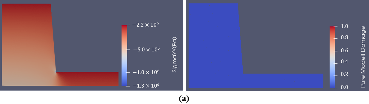
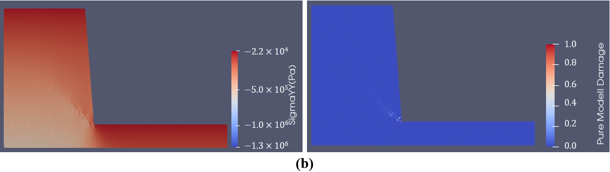
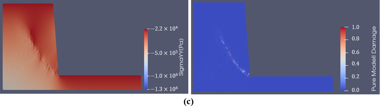
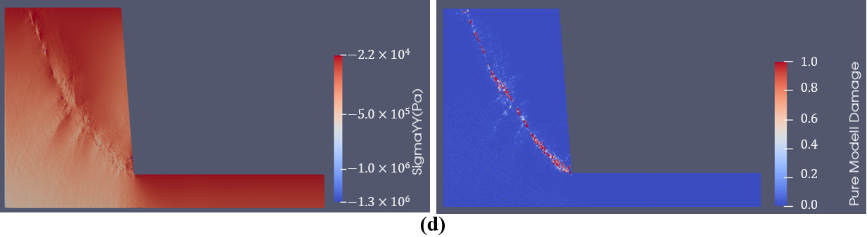
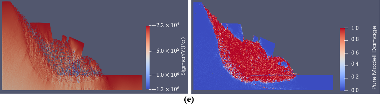
Figure 1. GPGUP-parallelized Y-HFDEM IDE modelling of rock slope failure process. (a) Stress equilibrium state; (b) 1 s; (c) 3 s; (d) 10 s; (e) 25 s.

The Figure 1 illustrates that the GPGUP-parallelized Y-HFDEM can effectively model the entire slope failure evolution process due to the implementation of the SRM in the proposed method. The GPGUP-parallelized FDEM with the implementation of SRM is a promising technique in the back analysis and prediction of the slope failure process, as it combined the advantages of the continuum methods and discontinuum methods, and it can naturally model the transition for rock from continuum to discontinuum through fracture and fragmentations.

References

  1. Abramson, L.W.; Lee, T.S.; Sharma, S.; Boyce, G.M. Slope Stability and Stabilization Methods; John Wiley & Sons: Hoboken, NJ, USA, 2001.
  2. Jin, Y.-F.; Yin, Z.-Y.; Yuan, W.-H. Simulating retrogressive slope failure using two different smoothed particle finite element methods: A comparative study. Eng. Geol. 2020, 279, 105870.
  3. Lv, Z.Q.; Wang, B.S.; Zhang, X.X. The PFC2DSimulation of the Slope Stability. In Advanced Materials Research; Trans Tech Publications Ltd.: Bäch SZ, Switzerland, 2015; pp. 240–243.
  4. Yang, Y.; Xu, D.; Liu, F.; Zheng, H. Modeling the entire progressive failure process of rock slopes using a strength-based criterion. Comput. Geotech. 2020, 126, 103726.
  5. Shen, J.; Karakus, M. Three-dimensional numerical analysis for rock slope stability using shear strength reduction method. Can. Geotech. J. 2014, 51, 164–172.
  6. Yodsomjai, W.; Keawsawasvong, S.; Thongchom, C.; Lawongkerd, J. Undrained stability of unsupported conical slopes in two-layered clays. Innov. Infrastruct. Solut. 2021, 6, 15.
  7. Yodsomjai, W.; Keawsawasvong, S.; Senjuntichai, T. Undrained stability of unsupported conical slopes in anisotropic clays based on anisotropic undrained shear failure criterion. Transp. Infrastruct. Geotechnol. 2021, 8, 557–568.
  8. Yodsomjai, W.; Keawsawasvong, S.; Likitlersuang, S. Stability of unsupported conical slopes in Hoek-Brown rock masses. Transp. Infrastruct. Geotechnol. 2021, 8, 279–295.
  9. Li, A.-J.; Lyamin, A.; Merifield, R. Seismic rock slope stability charts based on limit analysis methods. Comput. Geotech. 2009, 36, 135–148.
  10. Li, A.J.; Merifield, R.S.; Lyamin, A.V. Stability charts for rock slopes based on the Hoek-Brown failure criterion. Int. J. Rock Mech. Min. Sci. 2008, 45, 689–700.
  11. Jing, L. A review of techniques, advances and outstanding issues in numerical modelling for rock mechanics and rock engineering. Int. J. Rock Mech. Min. Sci. 2003, 40, 283–353.
  12. Jiang, M.; Murakami, A. Distinct element method analyses of idealized bonded-granulate cut slope. Granul. Matter 2012, 14, 393–410.
  13. Zhang, Y.; Xu, Q.; Chen, G.; Zhao, J.X.; Zheng, L. Extension of discontinuous deformation analysis and application in cohesive-frictional slope analysis. Int. J. Rock Mech. Min. Sci. 2014, 70, 533–545.
  14. Sun, L.; Liu, Q.; Abdelaziz, A.; Tang, X.; Grasselli, G. Simulating the entire progressive failure process of rock slopes using the combined finite-discrete element method. Comput. Geotech. 2022, 141, 104557.
  15. Zhou, W.; Yuan, W.; Ma, G.; Chang, X.L. Combined finite-discrete element method modeling of rockslides. Eng. Comput. 2016, 33, 1530–1559.
  16. Barla, M.; Piovano, G.; Grasselli, G. Rock slide simulation with the combined finite-discrete element method. Int. J. Geomech. 2012, 12, 711–721.
  17. Eberhardt, E.; Stead, D.; Coggan, J.S. Numerical analysis of initiation and progressive failure in natural rock slopes—The 1991 Randa rockslide. Int. J. Rock Mech. Min. Sci. 2004, 41, 69–87.
  18. Mahabadi, O.; Grasselli, G.; Munjiza, A. Y-GUI: A graphical user interface and pre-processor for the combined finite-discrete element code, Y2D, incorporating material heterogeneity. Comput. Geosci. 2010, 36, 241–252.
  19. An, H.; Wu, S.; Liu, H.; Wang, X. Hybrid Finite-Discrete Element Modelling of Various Rock Fracture Modes during Three Conventional Bending Tests. Sustainability 2022, 14, 592.
  20. An, H.; Song, Y.; Liu, H.; Han, H. Combined Finite-Discrete Element Modelling of Dynamic Rock Fracture and Fragmentation during Mining Production Process by Blast. Shock. Vib. 2021, 2021, 6622926.
  21. An, H.; Song, Y.; Liu, H. FDEM Modelling of Rock Fracture Process during Three-Point Bending Test under Quasistatic and Dynamic Loading Conditions. Shock. Vib. 2021, 2021, 5566992.
  22. An, H.; Liu, H.; Han, H. Hybrid finite–discrete element modelling of rock fracture process in intact and notched Brazilian disc tests. Eur. J. Environ. Civ. Eng. 2021, 1–34.
  23. Huaming, A.; Hongyuan, L.; Han, H. Hybrid finite-discrete element modelling of rock fracture during conventional compressive and tensile strength tests under quasi-static and dynamic loading conditions. Lat. Am. J. Solids Struct. 2020, 17, 1–32.
  24. An, H.; Liu, H.; Han, H. Hybrid Finite-Discrete Element Modelling of Excavation Damaged Zone Formation Process Induced by Blasts in a Deep Tunnel. Adv. Civ. Eng. 2020, 2020, 7153958.
  25. An, H.; Liu, H.; Han, H.; Zheng, X.; Wang, X. Hybrid finite-discrete element modelling of dynamic fracture and resultant fragment casting and muck-piling by rock blast. Comput. Geotech. 2017, 81, 322–345.
  26. Mohammadnejad, M.; Liu, H.; Chan, A.; Dehkhoda, S.; Fukuda, D. An overview on advances in computational fracture mechanics of rock. Geosystem Eng. 2021, 24, 206–229.
  27. Bradley, A.L. Investigating the Influence of Mechanical Anisotropy on the Fracturing Behavior of Brittle Clay Shales with Application to Deep Geological Repositories. In Proceedings of the 13th ISRM International Congress of Rock Mechanics, Montreal, QC, Canada, 10–13 May 2015.
  28. Zhao, Q.; Lisjak, A.; Mahabadi, O.; Liu, Q.; Grasselli, G. Numerical simulation of hydraulic fracturing and associated microseismicity using finite-discrete element method. J. Rock Mech. Geotech. Eng. 2014, 6, 574–581.
  29. Lukas, T.; Schiava D’Albano, G.G.; Munjiza, A. Space decomposition based parallelization solutions for the combined finite–discrete element method in 2D. J. Rock Mech. Geotech. Eng. 2014, 6, 607–615.
  30. Jing, L.; Hudson, J. Numerical methods in rock mechanics. Int. J. Rock Mech. Min. Sci. 2002, 39, 409–427.
  31. Munjiza, A. The Combined Finite-Discrete Element Method; Wiley Online Library: Hoboken, NJ, USA, 2004.
  32. Munjiza, A.; Xiang, J.; Garcia, X.; Latham, J.; D’Albano, G.S.; John, N. The virtual geoscience workbench, VGW: Open source tools for discontinuous systems. Particuology 2010, 8, 100–105.
  33. Vyazmensky, A.; Stead, D.; Elmo, D.; Moss, A. Numerical Analysis of Block Caving-Induced Instability in Large Open Pit Slopes: A Finite Element/Discrete Element Approach. Rock Mech. Rock Eng. 2010, 43, 21–39.
  34. Styles, T. Numerical Modelling and Analysis of Slope Stability within Fracture Dominated Rock Masses; University of Exeter: Exeter, UK, 2009.
  35. Tatonea, B.; Grassellia, G. A calibration procedure for two-dimensional laboratory-scale hybrid finite-discrete element simulations. Int. J. Rock Mech. Min. Sci. 2015, 75, 56–72.
  36. Mohammadi, S. Discontinuum Mechanics: Using Finite and Discrete Elements; WIT Press: Southampton, UK, 2003.
  37. Munjiza, A.; Andrews, K.; White, J. Combined single and smeared crack model in combined finite-discrete element analysis. Int. J. Numer. Methods Eng. 1999, 44, 41–57.
  38. Liu, H.; Kou, S.; Lindqvist, P.-A.; Tang, C. Numerical studies on the failure process and associated microseismicity in rock under triaxial compression. Tectonophysics 2004, 384, 149–174.
  39. Xiang, J.; Munjiza, A.; Latham, J.P. Finite strain, finite rotation quadratic tetrahedral element for the combined finite–discrete element method. Int. J. Numer. Methods Eng. 2009, 79, 946–978.
  40. Grasselli, G.; Lisjak, A.; Mahabadi, O.; Tatone, B. Slope Stability Analysis Using a Hybrid Finite-Discrete Element Method Code (EMDEM). In Proceedings of the 12th ISRM Congress, Beijing, China, 18–21 October 2011.
  41. An, H.; Fan, Y.; Liu, H. et al., The State of the Art and New Insight into Combined Finite–Discrete Element Modelling of the Entire Rock Slope Failure Process. Sustainability 2022, 14 (9), 4896.
More
Information
Subjects: Engineering, Civil
Contributors MDPI registered users' name will be linked to their SciProfiles pages. To register with us, please refer to https://encyclopedia.pub/register : , , ,
View Times: 783
Revisions: 3 times (View History)
Update Date: 09 May 2022
1000/1000
Video Production Service