Millimeter-Wave Radar Road Traffic Target Detection

Version	Summary	Created by	Modification	Content Size	Created at	Operation
1		Bo Yang	--	2432	2022-04-27 03:25:38	\|
2	update layout and references	Amina Yu	+ 1 word(s)	2433	2022-04-27 09:46:41	\| \|
3	update layout	Amina Yu	Meta information modification	2433	2022-04-29 07:13:43	\|

This entry is adapted from the peer-reviewed paper 10.3390/rs14081779

Using millimeter-wave radar as a monitoring system has raised increased in various fields attributed to its high detection accuracy and weather resistance. In road traffic applications, accurate acquisition of moving target information such as pedestrians and vehicles on the road is one of traffic radar’s most basic and essential tasks. With the development of intelligent transportation systems, the timely reflection of road conditions and realization of traffic accident warnings become necessary, which puts higher requirements on the low processing delay of radar systems.

millimeter-wave radar traffic surveillance moving target detection Monte Carlo simulation

1. Introduction

Generally, a number of approaches have been proposed to improve radar performance in traffic scenes, which can be mainly classified into two categories: (1) Around the signal processing direction, reduce or eliminate the interference signal as much as possible to ensure the purity of the target signal. (2) Design better detectors.

In the field of suppressing interference signals, cutting the interference-contaminated samples out of the signal is the most direct interference suppression method. Still, it also suppresses part of the valid signal of targets, resulting in less accurate reconstruction of the cutout samples of useful signals. To alleviate this effect, an iterative matrix-pencil (MP) method-based extrapolation for interference mitigation is proposed ^[1], but the accuracy of the reconstructed signal will decrease with the increase of the proportion of the contaminated samples. To improve signal reconstruction accuracy, an approach based on the sparse and low-rank decomposition of the Hankel matrix is proposed ^[2], however, iteration and best quality selection increase the complexity of the algorithm. For dealing with inter-radar interference, some new methods are proposed, such as designing a new orthogonal noise waveform ^[3] or presenting an interference mitigation technique in the tunable Q-factor wavelet transform (TQWT) domain ^[4]. In addition, some researchers have started from range and Doppler cell migration calibration to reduce signal distortion ^[5].

Designing better detectors is another direction to improve the application ability of radar. Compared with signal interference suppression, although the improvement of radar detection performance is weak, the design of the detector is more straightforward. In particular, in most cases, it will not add additional links and computational complexity, which is more suitable for low-cost radar systems with low-performance processors. So it is from the perspective of detector design. In the actual application of radar, the target always appears before the complex and changeable noise background, which is subject to changes in time and location, so the fixed threshold detection method cannot effectively distinguish the target from the background noise ^[6]. Radar Constant False Alarm Rate(CFAR) detection, which adaptively sets the detection threshold by evaluating current clutter environments ^[7]^[8], is a crucial technology for separating targets and background. Thus, an appropriate CFAR detection algorithm can improve radar detection performance and provide accurate target information for radar data processing. It also emerged as a key research aspect in radar detection.

The earliest proposed CFAR detection algorithm is the Cell Average CFAR (CA-CFAR) ^[9], which is based on the average local noise power level to detect targets. Design a reference window, take the window’s center unit as the candidate target, and use the amplitude accumulation value of other units in the window as the estimated value of background noise power. Whether the target exists is determined by judging the power value of the candidate target and the estimated noise power value. The CA-CFAR has poor detection performance under non-uniform noise and multi-target environments since interference signals or other targets within the reference window lead to background noise estimation error. Aiming at the problem of CA-CFAR detection performance degradation under multi-target or non-uniform noise, the maximum selection detection (GO-CFAR) ^[10] and the minimum selection detection (SO-CFAR) ^[11] are proposed. The GO-CFAR can maintain good false alarm control performance in a clutter edge environment, but ”target masking” in a multi-target environment will appear. The SO-CFAR has a good multi-target resolution ability, but its false alarm control ability is weak. Ordered Statistical CFAR (OS-CFAR) ^[12] is another typical CFAR detection method derived from the median filter concept in digital image processing. It arranges the sample units in the reference window according to the power value and selects one of the sample power values as the decision threshold. Compared with the detection performance of CA-CFAR, OS-CFAR has strong robustness to multi-target detection, but it has a high resulting CFAR loss. Some new methods combining OS and CA are proposed. Take the trimmed-mean detector (TM-CFAR) ^[13] algorithm as an example. The sample points in the reference window are sorted by amplitude value like OS-CFAR. Then remove part of the sample points with the largest and smallest amplitudes. Finally, the remaining sample points are averaged as the estimated value of background noise.

Now, new CFAR detection algorithms have been proposed based on traditional methods for different application requirements. Some scholars are dedicated to studying the multi-target detection capabilities of the detector. For example, the OSCA-CFAR algorithm is proposed, which combines the CA-CFAR algorithm and the OS-CFAR algorithm, to improve the multi-target detection capability of millimeter-wave radars, and gives algorithm performance simulation under an ideal noise environment ^[14]. Some researchers focus on improving the detection performance of the detector in a complex cluster environment. A Comp-CFAR method is proposed according to the central limit theorem and the logarithmic compression principle of the signal for targets detection in the clutter with long smearing effect characteristics ^[15]. A CFAR detector based on zlog(z) is used to reduce the false alarm rate in Weibull clutter ^[16]. Some other scholars have proposed a new method combined with machine learning ^[17]. Train a feedforward artificial neural network (ANN) on the data set containing the input and output of the CFAR sliding window to improve the efficiency of CFAR detection. However, this way increases the complexity of the algorithm.

Table 1 briefly summarizes the CFAR detection algorithms mentioned above. All current CFAR algorithms achieve target detection by designing a reference window and processing the data in the window. The design of the reference window can effectively reduce the level of clutter interference, but there are two drawbacks. One is that sliding the window reduces the efficiency of detecting objects. Especially in Linear Frequency Modulated Continuous Wave (LFMCW) radar systems, the input to the CFAR detector is a two-dimensional Range–Doppler Matrix (RDM). Although the principle of the CFAR algorithm has not changed, the sliding of the reference window has changed from a one-dimensional sliding search to a two-dimensional sliding search, which dramatically reduces the real-time performance of radar target detection. The other drawback is that the window limits the sample points for background noise estimation. Theoretically, the more sample points are used, the more accurate the estimated noise power value and the higher the CFAR detection accuracy. The design and sliding of the reference window limit the efficiency of radar target detection.

Table 1. A brief summary of the characteristics of CFAR algorithms.

CFAR Algorithms	Advantages	Disadvantages	Reference Window
CA-CFAR	High detection SNR in uniform noise	Low multi-target detection capability, High detection performance in non-uniform noise	YES
GO-CFAR	Good false alarm control in clutter edge	Low multi-target detection capability	YES
SO-CFAR	High multi-target detection capability	Low false alarm control ability	YES
OS-CFAR	Strong robustness to multi-target detection	High resulting CFAR loss	YES
OSCA-CFAR	High robust in multi-target situations, Low resulting CFAR loss	Performance degradation in non-pure noise situations	YES
Comp-CFAR	Suppression of clutter interference with long smearing effect characteristics	High algorithm complexity	YES
zlog(z)-CFAR	Reduce the false alarm rate in Weibull clutter	High algorithm complexity	YES
Machine learning	High detection accuracy	Low timeliness	YES

Fortunately, compared with the complex background environment such as the sea surface, the background noise in the traffic road is relatively simple. Especially when radar monitors moving targets, the effect of background noise data on detection can be eliminated using the de-zeroing Doppler method. Combining the non-ideal target motion (vehicle turning, braking and lane changing), the irregularity of the target reflection area, and the independence of the frame data, it was considered that the moving target echoes in the traffic road obey the ideal Swerling II model. Based on the above analysis, a reference window designed for complex noise and interference reduction may not be necessary for road traffic monitoring applications where the background noise is relatively clean. Instead, the sliding window increases the algorithm’s time complexity and reduces the efficiency of radar monitoring. To meet the requirement of low processing latency for traffic monitoring radar systems, it was proposed a CFAR algorithm based on the Monte Carlo to improve radar detection efficiency and sensitivity to moving targets in the traffic environment. Compared with the traditional algorithm, the algorithm has higher detection sensitivity and, more importantly, does not require the design and sliding of the reference window, which dramatically reduces the algorithm time complexity and improves the detection speed and efficiency. The contribution are summarized as follows: First, in the proposed CFAR detection algorithm, the entire RDM matrix area is randomly sampled to obtain the sample points of the background noise power estimation at the current moment. The principle is converting the Monte Carlo simulation principle, which gets properties of unknown quantities by independently repeating experiments, into a random sampling of the RDM matrix domain. This way breaks through the limitation of the reference window and can increase a large number of sample points for background noise estimation. Second, an interference point filtering method improves the accuracy of background noise estimation. Sort and filter the sample points according to the amplitude value of the sample points to remove possible target points or interference points. Then, the background noise estimated power value is obtained by the mean method. Finally, the target points in the RDM matrix are extracted by the background noise estimate. In addition, the parameter setting method of the algorithm is given, for example, according to the current physical platform and application environment, algorithm parameter values are obtained through repeated statistics. The configuration parameter process only needs to be executed once when the radar system environment is unchanged. Compared with the conventional method, simulations and practical experiments show that the method has higher detection sensitivity, higher detection accuracy, and lower detection latency, which improve radar detection efficiency in traffic surveillance.

2. Traffic Scene

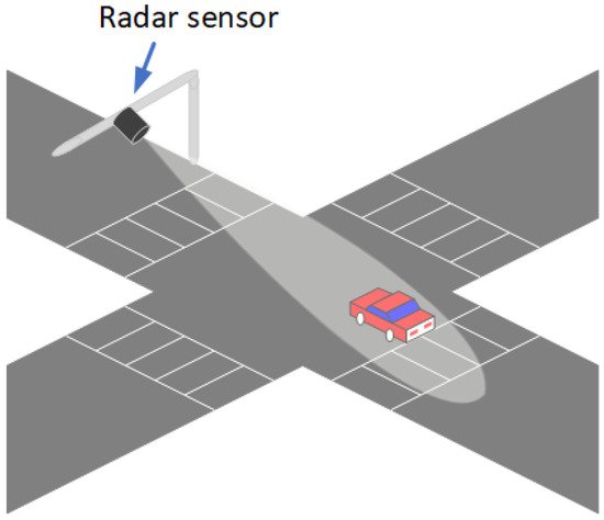
Usually, traffic sensors are installed on both sides of the road or on a fixed bracket extending to the center of the road (as shown in Figure 1), and they are required to have the following essential functions:

Figure 1. Traffic road scene.

High detection sensitivity. All targets in the field of view can be completely detected, including partial occlusion of the target;
Low information delay capability. It can reflect road conditions in real-time, i.e., the delay between data acquisition and road conditions output is required to be as short as possible (ideally, the delay should not exceed 100 ms);
Weather resistance. The sensor shall minimize the impact caused by night, fog, and other weather.

Millimeter-wave radar is considered to have the potential to be used in urban traffic monitoring since not affected by the environment, has high range resolution, and has low application cost. The CFAR detector as a vital part of radar target extraction has been extensively studied. By studying the traditional CFAR algorithm and analyzing the characteristics of the traffic environment, it were given a new CFAR detection algorithm to improve the sensitivity of radar to target detection, multi-target detection ability, and reduce delay, hoping it provides a unique reference for enhancing the adaptability of the radar in urban traffic monitoring.

3. Radar Background Noise Analysis in Traffic Scenea

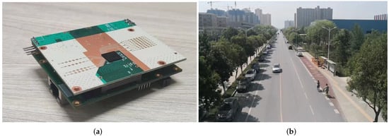
The radar chip (CAL77S244) based Radio Frequency(RF) front-end with three transmitting and four receiving antennas is used to transmit millimeter-wave and receive target echo signals. Additionally, a four-channel high-speed ADC is used for data acquisition. Finally, digital processing algorithms and extraction of target information are implemented on a back-end baseband processing system based on FPGA and ARM architecture. The data acquisition scene and radar system are shown in Figure 2.

Figure 2. (a) Radar system. (b) Data collection scenario.

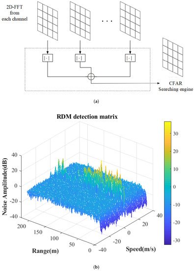
Figure 3 illustrates background noise data collection and display. Figure 3a is a flow chart of constant false alarm detection data acquisition. In this radar system, four receiving channels receive the radar’s electromagnetic echoes in the background environment and obtain the RDM matrix through incoherent accumulation. Figure 3b shows the distribution of the power amplitude of the RDM under the condition with no moving targets. The power amplitude value is abrupt and uneven in the zero-Doppler region (stationary objects region), which is caused by a combination of factors such as the number of objects at different distances and the size of the object’s reflection area. Preliminary observation shows that the noise power is distributed evenly in the non-zero Doppler domain (moving targets region), and there is no apparent abrupt change. In addition, the power of stationary objects does not significantly extend to the area where the moving targets are located.

Figure 3. (a) RDM data acquisition process. (b) Data collection scenario.

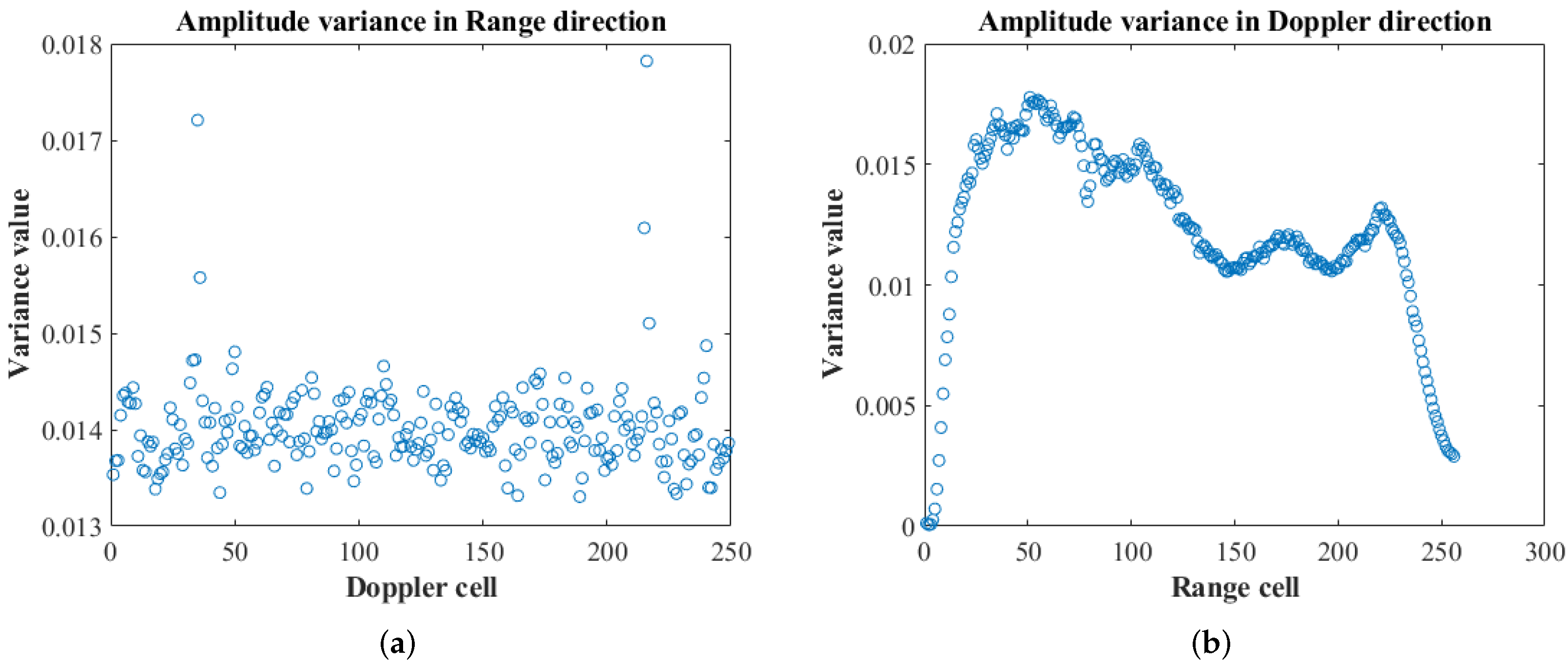
A distance dimension and velocity dimension data variance were used, an effective method to measure the degree of data dispersion, to evaluate the distribution of noise power amplitudes in the moving target area in the RDM matrix. It was counted the variance of each row (velocity dimension) or column (distance dimension) of the dataset in RDM as shown in Figure 4 (average of multiple statistics). It is worth noting that before calculating the variance, taking the average speed of pedestrians as a reference (0.5 m/s), it was eliminated that the cells where the static object is located in the RDM matrix, for example, cells with speed below 0.5 m/s. Both the variance of the velocity dimension and the variance of the distance dimension are less than 0.018, which could be thought that the background noise power amplitude is relatively uniform in the non-zero Doppler domain.

Figure 4. Background noise amplitude dispersion in RDM matrix (a) Noise amplitude variance in range direction. (b) Noise amplitude variance in Doppler direction.

The power density distribution is given as another characteristic of background noise. Previously, it was assumed that the radar noise distribution satisfies the Rayleigh distribution:

where

is the Rayleigh distribution parameter. The non-zero Doppler cells in RDM are sampled and processed by MATLAB Distribution Fitter Toolbox, and then the distribution of data (purple) and the fitting curve of Rayleigh distribution (red) are shown in Figure 5a. Figure 5b shows the matching degree between data probability distribution and Rayleigh distribution, i.e., the closer the data is to a curve line, the more consistent it is with Rayleigh distribution.

Figure 5. Simulation and fitting experiment example of RDM matrix noise density function (a) Noise distribution curve. (b) Matching degree of Rayleigh distribution.

References

Wang, J.; Ding, M.; Yarovoy, A. Matrix-Pencil Approach-Based Interference Mitigation for FMCW Radar Systems. IEEE Trans. Microw. Theory Tech. 2021, 69, 5099–5115.
Wang, J.; Ding, M.; Yarovoy, A. Interference Mitigation for FMCW Radar With Sparse and Low-Rank Hankel Matrix Decomposition. IEEE Trans. Signal Process. 2022, 70, 822–834.
Xu, Z.; Shi, Q. Interference Mitigation for Automotive Radar Using Orthogonal Noise Waveforms. IEEE Geosci. Remote Sens. Lett. 2018, 15, 137–141.
Xu, Z.; Yuan, M. An Interference Mitigation Technique for Automotive Millimeter Wave Radars in the Tunable Q-Factor Wavelet Transform Domain. IEEE Trans. Microw. Theory Tech. 2021, 69, 5270–5283.
Xu, Z.; Baker, C.J.; Pooni, S. Range and Doppler Cell Migration in Wideband Automotive Radar. IEEE Trans. Veh. Technol. 2019, 68, 5527–5536.
Moustafa, A.; Ahmed, F.M.; Moustafa, K.H.; Halwagy, Y. A new CFAR processor based on guard cells information. In Proceedings of the 2012 IEEE Radar Conference, Atlanta, GA, USA, 7–11 May 2012; pp. 133–137.
Farina, A.; Studer, F.A. A review of CFAR detection techniques in radar systems. Microw. J. 1986, 29, 115.
Gandhi, P.; Kassam, S. Analysis of CFAR processors in nonhomogeneous background. IEEE Trans. Aerosp. Electron. Syst. 1988, 24, 427–445.
Finn, H.M. Adaptive detection mode with threshold control as a function of spatially sampled-clutter-level estimates. RCA Rev. 1968, 29, 414–465.
Trunk, G. Range Resolution of Targets Using Automatic Detectors. IEEE Trans. Aerosp. Electron. Syst. 1978, AES-14, 750–755.
Pace, P.; Taylor, L. False alarm analysis of the envelope detection GO-CFAR processor. IEEE Trans. Aerosp. Electron. Syst. 1994, 30, 848–864.
Rohling, H. Radar CFAR Thresholding in Clutter and Multiple Target Situations. IEEE Trans. Aerosp. Electron. Syst. 1983, AES-19, 608–621.
Blake, S. OS-CFAR theory for multiple targets and nonuniform clutter. IEEE Trans. Aerosp. Electron. Syst. 1988, 24, 785–790.
Yan, J.; Li, X.; Shao, Z. Intelligent and fast two-dimensional CFAR procedure. In Proceedings of the 2015 IEEE International Conference on Communication Problem-Solving (ICCP), Guilin, China, 16–18 October 2015; pp. 461–463.
Liu, Y.; Zhang, S.; Suo, J.; Zhang, J.; Yao, T. Research on a New Comprehensive CFAR (Comp-CFAR) Processing Method. IEEE Access 2019, 7, 19401–19413.
Gouri, A.; Mezache, A.; Oudira, H. Radar CFAR detection in Weibull clutter based on zlog(z) estimator. Remote Sens. Lett. 2020, 11, 581–589.
Carretero, M.V.i.; Harmanny, R.I.A.; Trommel, R.P. Smart-CFAR, a machine learning approach to floating level detection in radar. In Proceedings of the 2019 16th European Radar Conference (EuRAD), Paris, France, 2–4 October 2019; pp. 161–164.

© Text is available under the terms and conditions of the Creative Commons Attribution (CC BY) license; additional terms may apply. By using this site, you agree to the Terms and Conditions and Privacy Policy.

Upload a video for this entry

Information

Subjects: Engineering, Electrical & Electronic

Contributors MDPI registered users' name will be linked to their SciProfiles pages. To register with us, please refer to https://encyclopedia.pub/register :

Bo Yang

Zhang Hua

View Times: 777

Update Date: 29 Apr 2022

Table of Contents

Video Upload Options

Confirm

1. Introduction

2. Traffic Scene

3. Radar Background Noise Analysis in Traffic Scenea

References