Visual-SLAM Algorithms

Version	Summary	Created by	Modification	Content Size	Created at	Operation
1		Andréa Macario Barros	+ 3757 word(s)	3757	2022-02-18 06:54:47	\|
2	Adjust the reference format	Lindsay Dong	-17 word(s)	3740	2022-03-23 02:29:46	\|

This entry is adapted from the peer-reviewed paper 10.3390/robotics11010024

The visual-based simultaneous localization and mapping (SLAM) techniques use one or more cameras in the sensor system, receiving 2D images as the source of information. In general, the visual-based SLAM algorithms are divided into three main threads: initialization, tracking, and mapping.

embedded SLAM RGB-D SLAM visual-inertial SLAM visual-SLAM

1. Introduction

Simultaneous localization and mapping (SLAM) technology, first proposed by Smith in 1986 ^[1], is used in an extensive range of applications, especially in the domain of augmented reality (AR) ^[2]^[3]^[4] and robotics ^[5]^[6]^[7]. The SLAM process aims at mapping an unknown environment and simultaneously locating a sensor system in this environment through the signals provided by the sensor(s). In robotics, the construction of a map is a crucial task, since it allows the visualization of landmarks, facilitating the environment’s visualization. In addition, it can help in the state estimation of the robot, relocating it, and decreasing estimation errors when re-visiting registered areas ^[8].

The map construction comes with two other tasks: localization and path planning. According to Stachniss ^[9], the mapping problem may be described by examining three questions considering the robot’s perspective: What does the world look like? Where am I? and How can I reach a given location? The first question is clarified by the mapping task, which searches to construct a map, i.e., a model of the environment. To do so, it requires the location of the observed landmarks, i.e., the answer for the second question, provided by the localization task. The localization task searches to determine the robot’s pose, i.e., its orientation and position and, consequently, locates the robot on the map. Depending on the first two tasks, the path planning clears up the last question, and seeks to estimate a trajectory for the robot to achieve a given location. It relies on the current robot’s pose, provided by the localization task, and on the environment’s characteristics, provided by the mapping task. SLAM is a solution that integrates both the mapping and localization tasks.

Visual-based SLAM algorithms can be considered especially attractive, due to their sensor configuration simplicity, miniaturized size, and low cost. The visual-based approaches can be divided into three main categories: visual-only SLAM, visual-inertial (VI) SLAM, and RGB-D SLAM. The first one refers to the SLAM techniques based only on 2D images provided by a monocular or stereo camera. They present a higher technical difficulty due to their limited visual input ^[10]. The robustness in the sensor’s tracking of the visual-SLAM algorithms may be increased by adding an inertial measurement unit (IMU), which can be found in their miniaturized size and low cost, while achieving high accuracy, essential aspects to many applications that require lightweight design, such as autonomous race cars ^[11]. In addition, visual-based SLAM systems may employ a depth sensor and process the depth information by applying a RGB-D-based approach.

2. Visual-Based SLAM

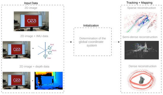
Figure 1 shows a general view of the three main parts generally present in visual-based SLAM approaches.

Figure 1. General components of a visual-based SLAM. The depth and inertial data may be added to the 2D visual input to generate a sparse map (generated with the ORB-SLAM3 algorithm ^[12] in the MH_01 sequence ^[13]), semi-dense map (obtained with the LSD-SLAM ^[14] in the dataset provided by the authors), and a dense reconstruction (Reprinted from ^[15]).

2.1. Visual-Only SLAM

The visual-only SLAM systems are based on 2D image processing. After the images’ acquisition from more than one point of view, the system performs the initialization process to define a global coordinate system and reconstruct an initial map. In the feature-based algorithms relying on filters (filtering-based algorithms), the first step consists of initializing the map points with high uncertainty, which may converge later to their actual positions. This procedure is followed by tracking, which attempts to estimate the camera pose. Simultaneously, the mapping process includes new points in the 3D reconstruction as more unknown scenes are observed.

2.1.1. Feature-Based Methods

SLAM algorithms based on features consider a certain number of points of interest, called keypoints. They can be detected in several images and matched by comparing their descriptors; this process provides the camera pose estimation information. The descriptor data and keypoint location compose the feature, i.e., the data used by the algorithm to process the tracking and mapping. As the feature-based methods do not use all the frame information, they are suitable to figure in embedded implementations. However, the feature extraction may fail in a textureless environment ^[16], as well as it generates a sparse map, providing less information than a dense one.

2.1.2. Direct Methods

In contrast with the feature-based methods, the direct methods use the sensor data without pre-processing, considering pixels’ intensities, and minimizing the photometric error. There are many different algorithms based on this methodology, and depending on the chosen technique, the reconstruction may be dense, semi-dense, or sparse. The reconstruction density is a substantial constraint to the algorithm’s real-time operation, since the joint optimization of both structure and camera positions is more computationally expensive for dense and semi-dense reconstructions than for a sparse one ^[17]. Figure 2 shows the main difference between feature-based (indirect) and direct methods according to their front-end and back-end, that is, the part of the algorithm responsible for sensor’s data abstraction and the part responsible for the interpretation of the abstracted data, respectively.

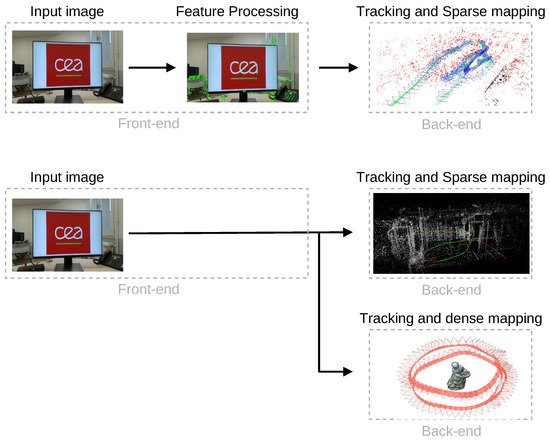
Figure 2. General differences between feature-based and direct methods. Top: main steps followed by the feature-based methods, resulting in a sparse reconstruction (map generated with the ORB-SLAM3 algorithm ^[12] in the MH_01/EuRoC sequence ^[13]). Bottom: main steps followed by a direct method, that may result in a sparse (generated from the reconstruction of sequence_02/TUM MonoVO ^[18] with the DSO algorithm ^[19]) or dense reconstruction (Reprinted from ^[15]), according to the chosen technique.

2.2. Visual-Inertial SLAM

The VI-SLAM approach incorporates inertial measurements to estimate the structure and the sensor pose. The inertial data are provided by the use of an inertial measurement unit (IMU), which consists of a combination of gyroscope, accelerometer, and, additionally, magnetometer devices. This way, the IMU is capable of providing information relative to the angular rate (gyroscope) and acceleration (accelerometer) along the x-, y-, and z-axes, and, additionally, the magnetic field around the device (magnometer). While adding an IMU may increase the information richness of the environment and provide higher accuracy, it also increases the algorithm’s complexity, especially during the initialization step, since, besides the initial estimation of the camera pose, the algorithm also has to estimate the IMU poses. VI-SLAM algorithms can be divided according to the type of fusion between the camera and IMU data, which can be loosely or tightly coupled. The loosely coupled methods do not merge the IMU states to estimate the full pose: instead, the IMU data are used to estimate the orientation and changes in the sensor’s position ^[20]. On the other side, the tightly coupled methods are based on the fusion of camera and IMU data into a motion equation, resulting in a state estimation that considers both data.

2.3. RGB-D SLAM

SLAM systems based on RGB-D data started to attract more attention with the advent of Microsoft’s Kinect in 2010. RGB-D sensors consist of a monocular RGB camera and a depth sensor, allowing SLAM systems to directly acquire the depth information with a feasible accuracy accomplished in real-time by low-cost hardware. As the RGB-D devices directly provide the depth map to the SLAM systems, the general framework of SLAM based on this approach differs from the other ones already presented.

Most of the RGB-D-based systems make use of the iterative closest point (ICP) algorithm to locate the sensor, fusing the depth maps to obtain the reconstruction of the whole structure. RGB-D systems present advantages such as providing color image data and dense depth map without any pre-processing step, hence decreasing the complexity of the SLAM initialization ^[10]. Despite this, this approach is most suitable to indoor environments, and requires large memory and power consumption ^[21].

3. Visual-SLAM Algorithms

Considering the general approach of the SLAM systems, six criteria that influence system dimensioning, accuracy, and hardware implementation were established. They are: algorithm type, map density, global optimization, loop closure, availability, and embedded implementations:

Algorithm type: this criterion indicates the methodology adopted by the algorithm. For the visual-only algorithms, it divided into feature-based, hybrid, and direct methods. Considering the visual-inertial algorithms, they must be filtering-based or optimization-based methods. Lastly, the RGB-D approach can be divided concerning their tracking method, which can be direct, hybrid, or feature-based.
Map density: in general, dense reconstruction requires more computational resources than a sparse one, having an impact on memory usage and computational cost. On the other hand, it provides a more detailed and accurate reconstruction, which may be a key factor in a SLAM project.
Global optimization: SLAM algorithms may include global map optimization, which refers to the technique that searches to compensate the accumulative error introduced by the camera movement, considering the consistency of the entire structure.
Loop closure: the loop closing detection refers to the capability of the SLAM algorithm to identify the images that were previously detected by the algorithm to estimate and correct the drift accumulated during the sensor movement.
Availability: several SLAM algorithms are open source and made available by the authors or have their implementations made available by third parties, facilitating their usage and reproduction.
Embedded implementations: the embedded SLAM implementation is an emerging field used in several applications, especially in robotics and automobile domains. This criterion depends on each algorithm’s hardware constraints and specificity, since there must be a trade-off between algorithm architecture in terms of energy consumption, memory, and processing usage.

3.1. Visual-Only SLAM

3.1.1. MonoSLAM (2007)

The first monocular SLAM algorithm is MonoSLAM, which was proposed by Davidson et al. ^[22] in 2007. The first step of the algorithm consists of the system’s initialization. Then, it updates the state vector considering a constant velocity motion model, where the camera motion and environment structure are estimated in real-time using an extended Kalman filter (EKF). The algorithm is represented by Figure 3.

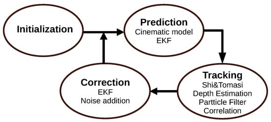
Figure 3. Diagram representing the MonoSLAM algorithm.

3.1.2. Parallel Tracking and Mapping (2007)

Another pioneer algorithm is the Parallel Tracking and Mapping (PTAM) ^[23] algorithm. PTAM was the first algorithm to separate Tracking and Mapping into two different threads and to apply the concept of keyframes to the mapping thread. First, the mapping thread performs the map initialization. New keyframes are added to the system as the camera moves and the initial map is expanded. Triangulation between two consecutive keyframes calculates the new point’s depth information. The tracking thread computes the camera poses, and for each new frame, it estimates an initial pose for performing the projection of the map points on the image. PTAM uses the correspondences to compute the camera pose by minimizing the reprojection error. Figure 4 represents the steps performed by the PTAM algorithm.

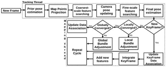
Figure 4. Diagram representing the PTAM algorithm.

3.1.3. Dense Tracking and Mapping (2011)

Dense tracking and mapping (DTAM), proposed by Newcombe et al. ^[24], was the first fully direct method in the literature. The algorithm is divided into two main parts: dense Mapping and dense tracking. The first stage searches to estimate the depth values by defining data cost volume representing the average photometric error of multiple frames computed for the inverse depth of the current frame. The inverse depth that minimizes the photometric error is selected to integrate the reconstruction. In the dense tracking stage, DTAM estimates the motion parameters by aligning an image from the dense model projected in a virtual camera and the current frame. Figure 5 shows a general view of the DTAM algorithm.

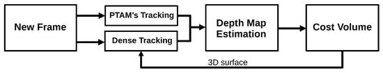
Figure 5. Diagram representing the DTAM algorithm.

3.1.4. Semi-Direct Visual Odometry (2014)

The semi-direct visual odometry (SVO) algorithm ^[25] combines the advantages of both feature-based and direct methods. The algorithm is divided into two main threads: motion estimation and mapping. The first thread searches to estimate the sensor’s motion parameters, which consists of minimizing the photometric error. The mapping thread is based on probabilistic depth filters, and it searches to estimate the optimum depth value for each 2D feature. When the algorithm achieves a low uncertainty, it inserts the 3D point in the reconstruction, as shown in Figure 6.

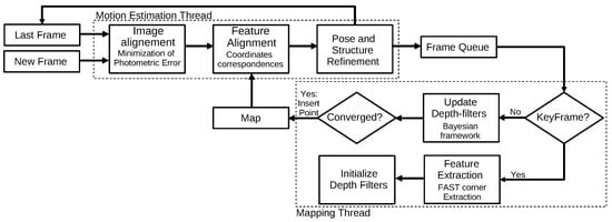
Figure 6. Diagram representing the SVO algorithm. Adapted from ^[25].

3.1.5. Large-Scale Direct Monocular SLAM (2014)

The large-scale direct monocular SLAM (LSD-SLAM) ^[14] is a direct algorithm that performs a semi-dense reconstruction. The algorithm consists of three main steps: tracking, depth map estimation, and map optimization. The first step minimizes the photometric error to estimate the sensor’s pose. Next, the LSD-SLAM performs the keyframe selection in the depth map estimation step. If it adds a new keyframe to the algorithm, it initializes its depth map; otherwise, it refines the depth map of the current keyframe by performing several small-baseline stereo comparisons. Finally, in the map optimization step, the LSD-SLAM incorporates the new keyframe in the map and optimizes it by applying a pose–graph optimization algorithm. Figure 7 illustrates the procedure.

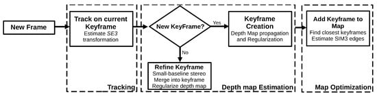
Figure 7. Diagram representing the LSD-SLAM algorithm. Adapted from ^[14].

3.1.6. ORB-SLAM 2.0 (2017)

The ORB-SLAM2 algorithm ^[26], originated from ORB-SLAM ^[27], is considered the state of the art of feature-based algorithms. It works in three parallel threads: tracking, local mapping, and loop closing. The first thread locates the sensor by finding features correspondences and minimizing the reprojection error. The local mapping thread is responsible for the map management operations. The last thread, loop closing, is in charge of detecting new loops and correcting the drift error in the loop. After processing the three threads, the algorithm also considers the whole structure and estimated motion consistency by performing a full bundle adjustment. Figure 8 represents the threads that constitute the algorithm.

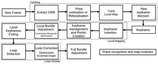
Figure 8. Diagram representing the ORB-SLAM 2.0 algorithm. Adapted from ^[27].

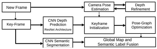
3.1.7. CNN-SLAM (2017)

CNN-SLAM ^[28] is one of the first works to present a real-time SLAM system based on convolutional neural networks (CNN). The algorithm may be divided into two different pipelines: one applied in every input frame and another in every keyframe. The first is responsible for the camera pose estimation by minimizing the photometric error between the current frame and the nearest keyframe. In parallel, for every keyframe, the depth is predicted by a CNN. In addition, the algorithm predicts the semantic segmentation for each frame. After these processing steps, the algorithm performs a pose-graph optimization to obtain a globally optimized pose estimation, as shown in Figure 9.

Figure 9. Diagram representing the CNN-SLAM algorithm. Adapted from ^[28].

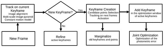
3.1.8. Direct Sparse Odometry (2018)

The direct sparse odometry (DSO) algorithm ^[19] combines a direct approach with a sparse reconstruction. The DSO algorithm considers a window of the most recent frames. It performs a continuous optimization by applying a local bundle adjustment that optimizes the keyframes window and the inverse depth map. The algorithm divides the image into several blocks and selects the highest intensity points. The DSO considers exposure time and lens distortion in the optimization to increase the algorithm’s robustness. Initially, this algorithm does not include global optimization or loop closure, but Xiang et al. ^[29] proposed an extension of the DSO algorithm, including loop closure detection and pose-graph optimization. The DSO main steps are represented in Figure 10.

Figure 10. Diagram representing the DSO algorithm.

3.2. Visual-Inertial SLAM

3.2.1. Multi-State Constraint Kalman Filter (2007)

The multi-state constraint Kalman filter (MSCKF) ^[30] can be implemented using both monocular and stereo cameras ^[31]. The algorithm’s pipeline consists of three main steps: propagation, image registration, and update. In the first step, the MSCKF considers the discretization of a continuous-time IMU model to obtain the propagation of the filter state and covariance. Then, the image registration performs the state augmentation each time a new image is recorded. This estimation is added in the state and covariance matrix to initiate the image processing module (feature extraction). Finally, the algorithm performs the filter update. Figure 11 represents the algorithm.

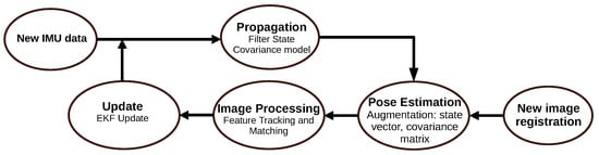
Figure 11. Diagram representing the MSCKF algorithm.

3.2.2. Open Keyframe-Based Visual-Inertial SLAM (2014)

Open Keyframe-based Visual-Inertial SLAM (OKVIS) ^[32] is an optimization-based method. It combines the IMU data and reprojection terms into an objective function, allowing the algorithm to jointly optimize both the weighted reprojection error and temporal error from IMU. The algorithm builds a local map, and then the subsequent keyframes are selected according to the keypoints match area. The algorithm can be depicted as shown in Figure 12.

Figure 12. Diagram representing the OKVIS algorithm.

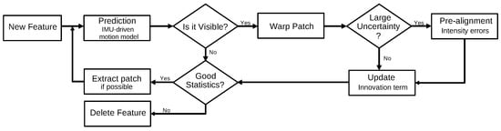
3.2.3. Robust Visual Inertial Odometry (2015)

The Robust Visual Inertial Odometry (ROVIO) algorithm ^[33] is another filter-based method that uses the EKF approach, and similar to other filter-based methods, it uses the IMU data to state propagation, and the camera data to filter update. However, besides performing the feature extraction, ROVIO executes the extraction of multi-level patches around the features, as illustrated by Figure 13.

Figure 13. Diagram representing the feature handling performed by the ROVIO algorithm. Adapted from ^[33].

3.2.4. Visual Inertial ORB-SLAM (2017)

The Visual-Inertial ORB-SLAM (VIORB) algorithm ^[34] is based on the already presented ORB-SLAM algorithm ^[26]. As such, the system also counts with three main threads: tracking, local mapping, and loop closing. In VIORB, the tracking thread estimates the sensor pose, velocity, and IMU biases. Additionally, this thread performs the joint optimization of the reprojection error of the matched points and IMU error data. The local mapping thread adopts a different culling policy considering the IMU operation. Finally, the loop closing thread implements a place recognition module to identify the keyframes already visited by the sensors. Furthermore, the algorithm performs an optimization to minimize the accumulated error. Figure 14 seeks to illustrate the main differences between the ORB-SLAM algorithm (see Figure 8) and its visual-inertial version.

Figure 14. Diagram representing the VIORB algorithm.

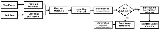
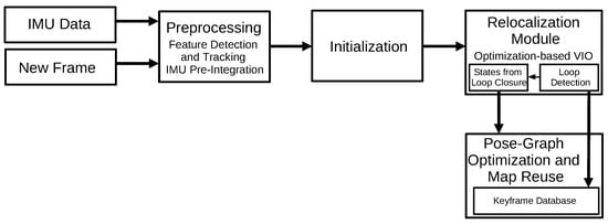
3.2.5. Monocular Visual-Inertial System (2018)

Monocular Visual-Inertial System (VINS-Mono) ^[35] is a monocular visual-inertial state estimator. It starts with a measurement process responsible for features extraction and tracking, and a pre-integration of the IMU data between the frames. Then, the algorithm performs an initialization process to provide the initial values for a non-linear optimization process that minimizes the visual and inertial errors. The VINS also implements a relocalization and a pose-graph optimization module that merges the IMU measurements and features observations. Figure 15 illustrates the VINS-Mono algorithm.

Figure 15. Diagram representing the VINS-Mono algorithm.

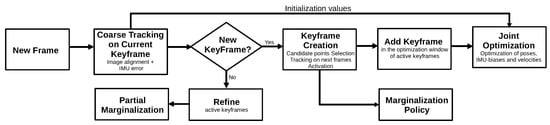
3.2.6. Visual-Inertial Direct Sparse Odometry (2018)

The Visual-Inertial Direct Sparse Odometry (VI-DSO) algorithm ^[36] is based on the already presented DSO algorithm ^[19]. The algorithm searches to minimize an energy function that combines the photometric and inertial errors, which is built considering a nonlinear dynamic model. Figure 16 shows an overview of the VI-DSO algorithm that illustrates its main differences concerning the DSO technique.

Figure 16. Diagram representing the VI-DSO algorithm.

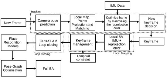
3.2.7. ORB-SLAM3 (2020)

ORB-SLAM3 algorithm ^[37] is a technique that combines the ORB-SLAM and VIORB algorithms. As with its predecessors, the algorithm is divided into three main threads: tracking, local mapping and, instead of loop closing, loop closing and map merging. In addition, ORB-SLAM3 maintains a multi-map representation called Atlas, which maintains an active map used by the tracking thread, and non-active maps used for relocalization and place recognition. The first two threads follow the same principle as VIORB, while map merging is added to the last thread. The loop closing and map merging thread uses all the maps in Atlas to identify common parts and perform loop correction or merge maps and change the active map, depending on the location of the overlapped area. Another important aspect of ORB-SLAM3 concerns the proposed initialization technique that relies on the Maximum-a-Posteriori algorithm individually applied to the visual and inertial estimations, which are later jointly optimized. This algorithm can be used with monocular, stereo, and RGB-D cameras, and implements global optimizations and loop closures techniques.

3.3. RGB-D SLAM

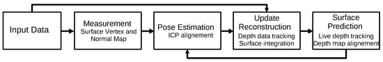
3.3.1. KinectFusion (2011)

The KinectFusion algorithm ^[38] was the first algorithm based on an RGB-D sensor to operate in real-time. The algorithm includes four main steps: the measurement, pose estimation, reconstruction update, and surface prediction. In the first step, the RGB image and depth data are used to generate a vertex and a normal map. In the pose estimation step, the algorithm applies the ICP alignment between the current surface and the predicted one (provided by the previous step). Then, the reconstruction update step integrates the new depth frame into the 3D reconstruction, which is raycasted into the new estimated frame to obtain a new dense surface prediction. The KinectFusion algorithm is capable of good mapping in maximum medium-sized rooms ^[38]. However, it accumulates drift errors, since it does not perform loop closing ^[39]. An overview of the steps performed by the algorithm is shown in Figure 17.

Figure 17. Diagram representing the KinectFusion algorithm. Adapted from ^[38].

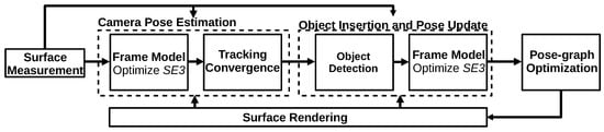
3.3.2. SLAM++ (2013)

The SLAM++ algorithm ^[40] is an object-oriented SLAM algorithm that takes advantage of previously known scenes containing repeated objects and structures, such as a classroom. After the system initialization, SLAM++ operates in four steps: camera pose estimation, object insertion, and pose update, pose–graph optimization, and surface rendering. The first step estimates the current camera pose by applying the ICP algorithm, considering dense multi-object prediction in the current SLAM graph. Next, the algorithm searches to identify objects in the current frame using the database information. The third step inserts the considered objects in the SLAM graph by performing a pose–graph optimization operation. Finally, the algorithm renders the objects in the graph, as shown in Figure 18. SLAM++ performs loop closure detection and, by considering the object’s repeatability, it increases its efficiency and scene description. Nevertheless, the algorithm is most suitable for already known scenes.

Figure 18. Diagram representing the SLAM++ algorithm. Adapted from ^[40].

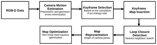
3.3.3. Dense Visual Odometry (2013)

The dense visual odometry SLAM (DVO-SLAM) algorithm, proposed by Kerl et al. ^[41], is a keyframe-based technique. It minimizes the photometric error between the keyframes to acquire the depth values and pixels coordinates, as well as camera motion. The algorithm calculates, for each input frame, an entropy value that is compared to a threshold value. The same principle is used for loop detection, although it uses a different threshold value. The map is represented by a SLAM graph where the vertex has camera poses, and edges are the transformations between keyframes. This algorithm is robust to textureless scenes and performs loop closure detection. The map representation relies on a representation of the keyframes, and the algorithm does not perform an explicit map reconstruction. Figure 19 shows an overview of the DVO algorithm.

Figure 19. Diagram representing the DVO algorithm.

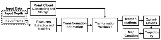
3.3.4. RGBDSLAMv2 (2014)

The RGBDSLAMv2 ^[42] is one of the most popular RGB-D-based algorithms and relies on feature extraction. It performs the RANSAC algorithm to estimate the transformation between the matched features and the ICP algorithm to obtain pose estimation. Finally, the system executes a global optimization and loop closure to eliminate the accumulated error. In addition, this method proposes using an environment measurement model (EMM) to validate the transformations obtained between the frames. The algorithm is based on SIFT features, which degrades its real-time performance. RGBDSLAMv2 presents a high computation consumption and requires a slow movement by the sensor for its correct operation ^[39]. Figure 20 represents the algorithm.

Figure 20. Diagram representing the RGBDSLAMv2 algorithm. Adapted from ^[42].

References

Smith, R.; Cheeseman, P. On the Representation and Estimation of Spatial Uncertainty. Int. J. Robot. Res. 1987, 5, 56–68.
Jinyu, L.; Bangbang, Y.; Danpeng, C.; Nan, W.; Guofeng, Z.; Hujun, B. Survey and evaluation of monocular visual-inertial SLAM algorithms for augmented reality. Virtual Real. Intell. Hardw. 2019, 1, 386–410.
Covolan, J.P.; Sementille, A.; Sanches, S. A mapping of visual SLAM algorithms and their applications in augmented reality. In Proceedings of the 2020 22nd Symposium on Virtual and Augmented Reality (SVR), Porto de Galinhas, Brazil, 7–10 November 2020.
Singandhupe, A.; La, H. A Review of SLAM Techniques and Security in Autonomous Driving. In Proceedings of the 2019 Third IEEE International Conference on Robotic Computing (IRC), Naples, Italy, 25–27 February 2019; pp. 602–607.
Dworakowski, D.; Thompson, C.; Pham-Hung, M.; Nejat, G. A Robot Architecture Using ContextSLAM to Find Products in Unknown Crowded Retail Environments. Robotics 2021, 10, 110.
Ruan, K.; Wu, Z.; Xu, Q. Smart Cleaner: A New Autonomous Indoor Disinfection Robot for Combating the COVID-19 Pandemic. Robotics 2021, 10, 87.
Liu, C.; Zhou, C.; Cao, W.; Li, F.; Jia, P. A Novel Design and Implementation of Autonomous Robotic Car Based on ROS in Indoor Scenario. Robotics 2020, 9, 19.
Cadena, C.; Carlone, L.; Carrillo, H.; Latif, Y.; Scaramuzza, D.; Neira, J.; Reid, I.; Leonard, J.J. Past, Present, and Future of Simultaneous Localization and Mapping: Toward the Robust-Perception Age. IEEE Trans. Robot. 2016, 32, 1309–1332.
Stachniss, C. Robotic Mapping and Exploration; Springer: Berlin/Heidelberg, Germany, 2009; Volume 55.
Taketomi, T.; Uchiyama, H.; Ikeda, S. Visual SLAM algorithms: A survey from 2010 to 2016. IPSJ Trans. Comput. Vis. Appl. 2017, 9, 1–11.
Kabzan, J.; Valls, M.; Reijgwart, V.; Hendrikx, H.; Ehmke, C.; Prajapat, M.; Bühler, A.; Gosala, N.; Gupta, M.; Sivanesan, R.; et al. AMZ Driverless: The Full Autonomous Racing System. J. Field Robot. 2020, 37, 1267–1294.
Campos, C.; Elvira, R.; Rodríguez, J.J.G.; Montiel, J.M.M.; D. Tardós, J. ORB-SLAM3: An Accurate Open-Source Library for Visual, Visual–Inertial, and Multimap SLAM. IEEE Trans. Robot. 2021, 37, 1874–1890.
Burri, M.; Nikolic, J.; Gohl, P.; Schneider, T.; Rehder, J.; Omari, S.; Achtelik, M.; Siegwart, R. The EuRoC micro aerial vehicle datasets. Int. J. Robot. Res. 2016, 35, 1157–1163.
Engel, J.; Schöps, T.; Cremers, D. LSD-SLAM: Large-Scale Direct Monocular SLAM. In Computer Vision–ECCV 2014; Fleet, D., Pajdla, T., Schiele, B., Tuytelaars, T., Eds.; Springer International Publishing: Cham, Switzerland, 2014; pp. 834–849.
Bianco, S.; Ciocca, G.; Marelli, D. Evaluating the Performance of Structure from Motion Pipelines. J. Imaging 2018, 4, 98.
Loo, S.Y.; Amiri, A.; Mashohor, S.; Tang, S.; Zhang, H. CNN-SVO: Improving the Mapping in Semi-Direct Visual Odometry Using Single-Image Depth Prediction. In Proceedings of the 2019 International Conference on Robotics and Automation (ICRA), Montreal, QC, Canada, 20–24 May 2019.
Boikos, K.; Bouganis, C.S. Semi-dense SLAM on an FPGA SoC. In Proceedings of the 2016 26th International Conference on Field Programmable Logic and Applications (FPL), Lausanne, Switzerland, 29 August–2 September 2016; pp. 1–4.
Engel, J.; Usenko, V.; Cremers, D. A Photometrically Calibrated Benchmark For Monocular Visual Odometry. arXiv 2016, arXiv:1607.02555.
Engel, J.; Koltun, V.; Cremers, D. Direct Sparse Odometry. IEEE Trans. Pattern Anal. Mach. Intell. 2018, 40, 611–625.
Chen, C.; Zhu, H.; Li, M.; You, S. A Review of Visual-Inertial Simultaneous Localization and Mapping from Filtering-Based and Optimization-Based Perspectives. Robotics 2018, 7, 45.
Canovas, B.; Rombaut, M.; Nègre, A.; Pellerin, D.; Olympieff, S. Speed and Memory Efficient Dense RGB-D SLAM in Dynamic Scenes. In Proceedings of the IROS 2020—IEEE/RSJ International Conference on Intelligent Robots and Systems, Las Vegas, NV, USA, 25–29 October 2020; pp. 4996–5001.
Davison, A.J.; Reid, I.D.; Molton, N.D.; Stasse, O. MonoSLAM: Real-Time Single Camera SLAM. IEEE Trans. Pattern Anal. Mach. Intell. 2007, 29, 1052–1067.
Klein, G.; Murray, D. Parallel Tracking and Mapping for Small AR Workspaces. In Proceedings of the 2007 6th IEEE and ACM International Symposium on Mixed and Augmented Reality, Nara, Japan, 13–16 November 2007; pp. 225–234.
Newcombe, R.A.; Lovegrove, S.J.; Davison, A.J. DTAM: Dense tracking and mapping in real-time. In Proceedings of the 2011 International Conference on Computer Vision, Barcelona, Spain, 6–13 November 2011; pp. 2320–2327.
Forster, C.; Pizzoli, M.; Scaramuzza, D. SVO: Fast semi-direct monocular visual odometry. In Proceedings of the 2014 IEEE International Conference on Robotics and Automation (ICRA), Hong Kong, China, 31 May–7 June 2014; pp. 15–22.
Mur-Artal, R.; Tardós, J.D. ORB-SLAM2: An Open-Source SLAM System for Monocular, Stereo, and RGB-D Cameras. IEEE Trans. Robot. 2017, 33, 1255–1262.
Mur-Artal, R.; Montiel, J.; Tardos, J. ORB-SLAM: A versatile and accurate monocular SLAM system. IEEE Trans. Robot. 2015, 31, 1147–1163.
Tateno, K.; Tombari, F.; Laina, I.; Navab, N. CNN-SLAM: Real-Time Dense Monocular SLAM with Learned Depth Prediction. In Proceedings of the 2017 IEEE Conference on Computer Vision and Pattern Recognition (CVPR), Honolulu, HI, USA, 21–26 July 2017; pp. 6565–6574.
Gao, X.; Wang, R.; Demmel, N.; Cremers, D. LDSO: Direct Sparse Odometry with Loop Closure. In Proceedings of the 2018 IEEE/RSJ International Conference on Intelligent Robots and Systems (IROS), Madrid, Spain, 1–5 October 2018.
Mourikis, A.I.; Roumeliotis, S.I. A Multi-State Constraint Kalman Filter for Vision-aided Inertial Navigation. In Proceedings of the 2007 IEEE International Conference on Robotics and Automation, Roma, Italy, 10–14 April 2007; pp. 3565–3572.
Sun, K.; Mohta, K.; Pfrommer, B.; Watterson, M.; Liu, S.; Mulgaonkar, Y.; Taylor, C.J.; Kumar, V. Robust Stereo Visual Inertial Odometry for Fast Autonomous Flight. IEEE Robot. Autom. Lett. 2018, 3, 965–972.
Leutenegger, S.; Lynen, S.; Bosse, M.; Siegwart, R.; Furgale, P. Keyframe-Based Visual-Inertial Odometry Using Nonlinear Optimization. Int. J. Robot. Res. 2014, 34, 314–334.
Bloesch, M.; Omari, S.; Hutter, M.; Siegwart, R. Robust visual inertial odometry using a direct EKF-based approach. In Proceedings of the 2015 IEEE/RSJ International Conference on Intelligent Robots and Systems (IROS), Hamburg, Germany, 28 September–3 October 2015; pp. 298–304.
Mur-Artal, R.; Tardós, J.D. Visual-Inertial Monocular SLAM With Map Reuse. IEEE Robot. Autom. Lett. 2017, 2, 796–803.
Qin, T.; Li, P.; Shen, S. VINS-Mono: A Robust and Versatile Monocular Visual-Inertial State Estimator. IEEE Trans. Robot. 2018, 34, 1004–1020.
Von Stumberg, L.; Usenko, V.; Cremers, D. Direct Sparse Visual-Inertial Odometry Using Dynamic Marginalization. In Proceedings of the 2018 IEEE International Conference on Robotics and Automation (ICRA), Brisbane, Australia, 21–25 May 2018; pp. 2510–2517.
Campos, C.; Montiel, J.M.; Tardós, J.D. Inertial-Only Optimization for Visual-Inertial Initialization. In Proceedings of the 2020 IEEE International Conference on Robotics and Automation (ICRA), Paris, France, 31 May–31 August 2020; pp. 51–57.
Newcombe, R.A.; Izadi, S.; Hilliges, O.; Molyneaux, D.; Kim, D.; Davison, A.J.; Kohi, P.; Shotton, J.; Hodges, S.; Fitzgibbon, A. KinectFusion: Real-time dense surface mapping and tracking. In Proceedings of the 2011 10th IEEE International Symposium on Mixed and Augmented Reality, Basel, Switzerland, 26–29 October 2011; pp. 127–136.
Jin, Q.; Liu, Y.; Man, Y.; Li, F. Visual SLAM with RGB-D Cameras. In Proceedings of the 2019 Chinese Control Conference (CCC), Guangzhou, China, 27–30 July 2019; pp. 4072–4077.
Salas-Moreno, R.F.; Newcombe, R.A.; Strasdat, H.; Kelly, P.H.; Davison, A.J. SLAM++: Simultaneous Localisation and Mapping at the Level of Objects. In Proceedings of the 2013 IEEE Conference on Computer Vision and Pattern Recognition, Portland, OR, USA, 23–28 June 2013; pp. 1352–1359.
Kerl, C.; Sturm, J.; Cremers, D. Dense visual SLAM for RGB-D cameras. In Proceedings of the 2013 IEEE/RSJ International Conference on Intelligent Robots and Systems, Tokyo, Japan, 3–7 November 2013; pp. 2100–2106.
Endres, F.; Hess, J.; Sturm, J.; Cremers, D.; Burgard, W. 3-D Mapping With an RGB-D Camera. IEEE Trans. Robot. 2014, 30, 177–187.

© Text is available under the terms and conditions of the Creative Commons Attribution (CC BY) license; additional terms may apply. By using this site, you agree to the Terms and Conditions and Privacy Policy.

Upload a video for this entry

Information

Subjects: Engineering, Electrical & Electronic

Contributor MDPI registered users' name will be linked to their SciProfiles pages. To register with us, please refer to https://encyclopedia.pub/register :

Andréa Macario Barros

View Times: 6.2K

Update Date: 23 Mar 2022

Table of Contents

Video Upload Options

Confirm