Your browser does not fully support modern features. Please upgrade for a smoother experience.
Submitted Successfully!
 +1 credit
Thank you for your contribution! You can also upload a video entry or images related to this topic.
For video creation, please contact our Academic Video Service.
| Version | Summary | Created by | Modification | Content Size | Created at | Operation |
|---|---|---|---|---|---|---|
| 1 | Andrey E. Krauklis | + 2220 word(s) | 2220 | 2022-01-11 03:10:34 | | | |
| 2 | Dean Liu | -6 word(s) | 2214 | 2022-03-15 04:30:18 | | |
Video Upload Options
We provide professional Academic Video Service to translate complex research into visually appealing presentations. Would you like to try it?
Cite
If you have any further questions, please contact Encyclopedia Editorial Office.
Krauklis, A. Environmental Ageing of Polymers and Polymer Composites. Encyclopedia. Available online: https://encyclopedia.pub/entry/20577 (accessed on 12 June 2026).
Krauklis A. Environmental Ageing of Polymers and Polymer Composites. Encyclopedia. Available at: https://encyclopedia.pub/entry/20577. Accessed June 12, 2026.
Krauklis, Andrey. "Environmental Ageing of Polymers and Polymer Composites" Encyclopedia, https://encyclopedia.pub/entry/20577 (accessed June 12, 2026).
Krauklis, A. (2022, March 15). Environmental Ageing of Polymers and Polymer Composites. In Encyclopedia. https://encyclopedia.pub/entry/20577
Krauklis, Andrey. "Environmental Ageing of Polymers and Polymer Composites." Encyclopedia. Web. 15 March, 2022.
Copy Citation
Polymers and polymer composites are often exposed to elevated temperatures, mechanical stress, water and humid air environments, where their performance is negatively impacted by environmental ageing, reducing their service lifetime.
polymer
fibre
composite
biodegradable
environmental ageing
durability
1. Introduction
Fibre-reinforced polymer (FRP) composites are widely used in structural applications in the wind energy sector, marine and offshore, oil and gas, transportation and aircraft industries, where a design lifetime of composite structures is typically 25 years or more [1]. Hence, modelling and predicting the extent of composite material property deterioration due to exposure to water, humidity (e.g., open sea or rain), and other environmental stressors and media is of great interest for both the designers and end-users of composite materials and structures [2].
In the state-of-the-art, qualification of new composite materials is achieved mainly with experimental validation [1][3]. Such testing programs involve incredibly high costs, in which the verification of new composite materials is required (involving a massive testing programme) [1]. Even the slightest change in material or structural design choice involves extremely high testing costs which often is the “bottleneck” for the projects [1][3]. Certification costs can be as high as aircraft development costs in aviation programs, higher than USD 100 M [4]. Merely certifying a new composite material for aviation can cost up to several million USD as shown by a USD 3.7 M project led by the Korean Civil Aviation Certification Agency [5]. Furthermore, the timeline for material development ranges from a few years to modify existing materials to 10–20 years for new materials [6]. For the automotive industry, development cycles last an average of 20–30 months, and the cost of testing a new composite material would be higher than EUR 500,000 [7]. DNV GL has led a Joint Industrial Project to study offshore and marine applications composites, estimating potential savings for $10 M [8]. For wind blades, the impact of material certification can be evaluated in a similar magnitude; a cost model has found material and labour cost to comprise almost 75% of the total price of a composite blade [9].
Mathematical modelling has become an essential aspect of such validation [3]. Qualification by simulation, based on fundamental scientific principles, can substantially reduce the qualification costs. Thus, modelling tools are the future for the successful development of the polymer composite industry [1]. The current direction in the composite industry is to replace testing as much as possible with durability prediction models [1][10].
2. Emerging Trends in Degradation Modelling of Biodegradable Polymers
2.1. Biodegradation—An Introduction to Terms and Definitions
Plastics can be divided into four characteristic groups. A two-axis model has been used most often in the literature. The vertical axis shows the biodegradability of plastics, whereas the horizontal axis represents the material origin (petrochemical or renewable raw materials). In addition to non-biodegradable plastics made from petrochemical raw materials (classic or traditional plastics), biodegradable plastics are made from renewable raw materials. These are plastics that have been produced from biomass-containing raw materials and are biodegradable. Furthermore, biodegradable plastics that can be biodegraded were produced from fossil raw materials. Finally, there are the non-biodegradable plastics made from renewable raw materials produced from biomass but are not biodegradable [11]. According to an ASTM definition, biodegradable polymers and plastics are materials that can be quantitatively converted to either carbon dioxide and water or methane and water under aerobic and anaerobic conditions [12].
Biodegradable polymers (e.g., polyesters, polyamines) have a higher concentration of heteroatoms than fossil-based polymers with pure carbon backbones, such as polyethylene. Furthermore, biodegradable polymers are often derived from raw materials inferior to their petroleum-based counterparts [13].
There are usually three stages (fragmentation, hydrolysis and assimilation) that are part of the biodegradation process in enzymatic hydrolysis. Microbial secretases catalyse this process. In the first step, small pieces (microplastic particles) are formed by weathering, UV-irradiation, mechanical forces and microorganisms. Subsequent hydrolysis at the ester bond of the polymer results in the reduction of molecular mass and the formation of soluble monomers and oligomers. These breakdown products are taken up by intracellular enzymes and used as a carbon and energy source to produce a greater cell biomass and end products such as carbon dioxide and water. This is called the assimilation process (see Figure 1, [14]).
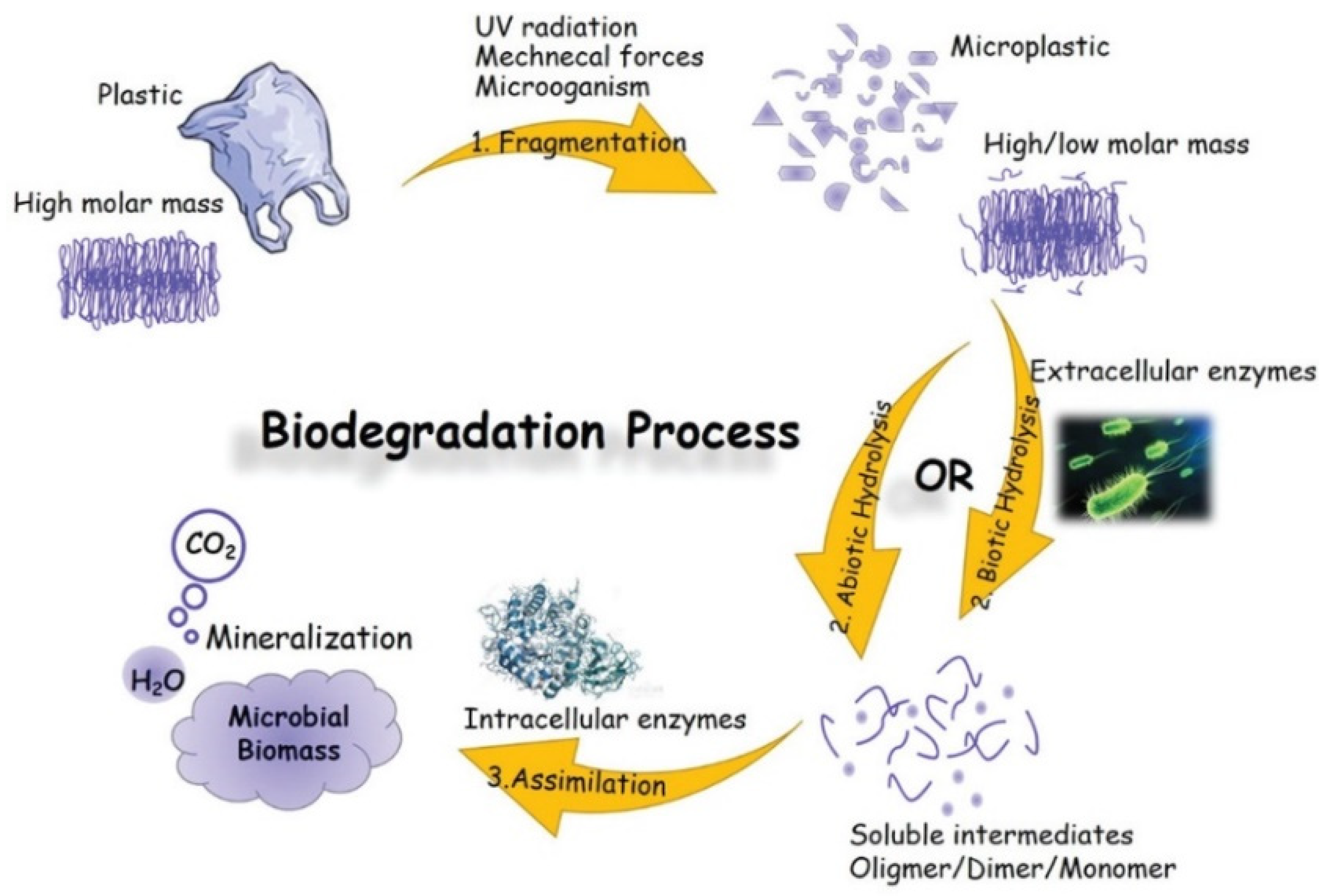
Figure 1. The different steps are involved in the biodegradation process [14].
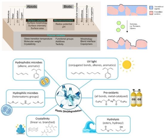
The hydrolysis of the polymer can be either biotic or abiotic, with abiotic hydrolysis being much slower than biotic or enzymatic hydrolysis [15][16]. In a natural environment, both biotic and abiotic factors synergistically influence biodegradable polymers with respect to compositions and processes [13][17][18]. Several aspects influence the microenvironment, such as pH, redox potential, interfacial chemistry and physics, chemical composition, crystallinity, and polydispersity [13]. Figure 2 left shows the interaction of abiotic and biotic factors and the interplay of microorganisms such as bacteria, fungi, archaea and algae [19], environment and the polymer as a complex multivariable space of biodegradation. The movement of the polymer chains becomes restricted with increased crystallisation. As a result, fewer polymer chains are available for degradation products such as microbial lipases or other ester-cleaving molecules. Previous studies have shown that the degradation of PHBV (poly(hydroxybutyrate-co-valerate)), catalysed by lipases, occurs preferentially in the amorphous regions [20]. As shown on the right in Figure 2, the microbial enzymes are thus only able to degrade the amorphous regions of the polymer. The adjacent crystalline regions limit the depth of degradation. Essential factors and chemical groups impaired during the biodegradation process are shown at the bottom of Figure 2 [21]. Hydrophilic microbes usually have higher degradation rates than hydrophobic microbes, as was demonstrated in the literature [22].
2.2. Data-Driven Approach to Elucidate Degradation Trends
Min et al. addressed the question as to how many descriptors would be needed to model the degradation behaviour of plastics in the ocean or to understand if degradation is possible. They present a so-called data-driven approach to investigate the degradation trends of plastic debris. The biotic and abiotic degradation behaviour in seawater is linked to physical properties and molecular structures [17]. Figure 3 exhibits the flow chart to calculate the hydrophobicity. It is based on a molecular level method combining theory, simulation, and experimental validation [24].
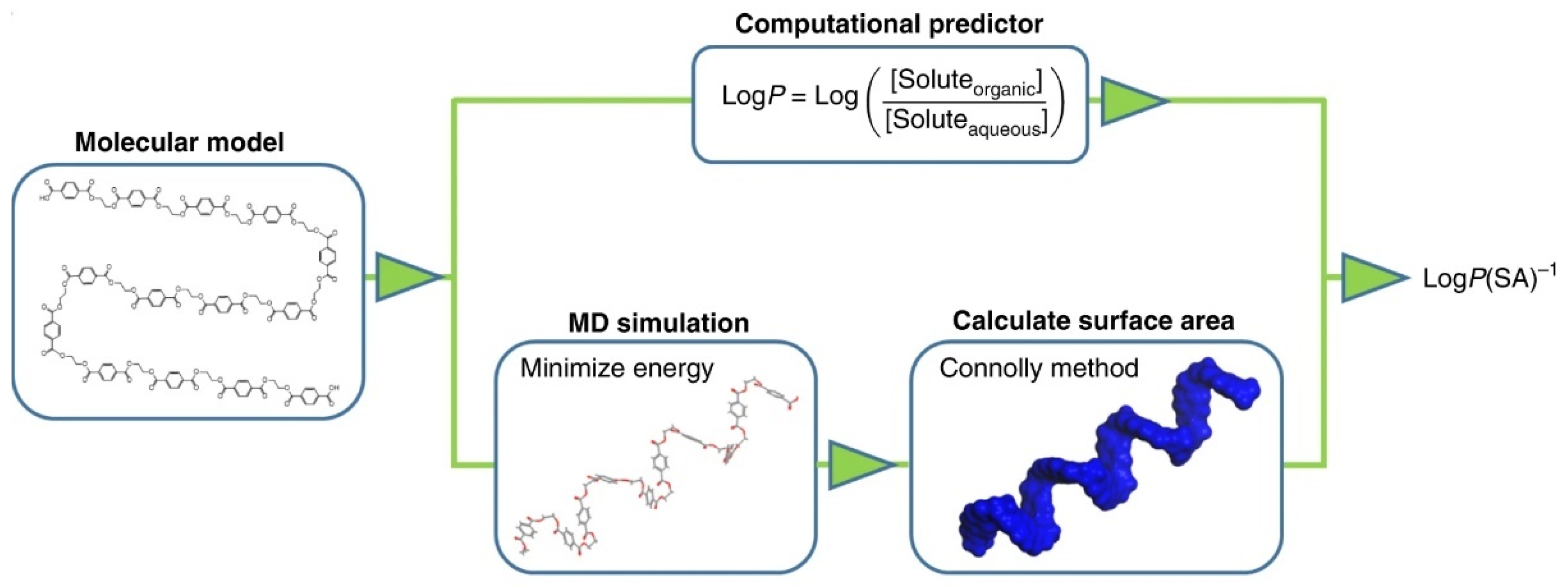
Figure 3. Flow chart for calculating hydrophobicity [17].
Here, negative LogP values predict water solubility, for polymers that swell in water or polymers that tend to absorb moisture. Positive values, on the other hand, predict insolubility. Different polymers can be compared by using MD (molecular dynamics simulation) to minimise the energy of molecular models and then calculating the surface area (SA) [17].
The wide range of hydrophobicity of plastics is revealed in Figure 4 [17]. Water-soluble plastics (see blue colour) such as PEG (polyethylene glycol) or PVA (polyvinyl alcohol) exhibit polar groups such as OH groups degrading via microbial oxidation [25]. In the second category (yellow colour), the erosion tendency of the polyester surface correlates with hydrophobicity when Tg values are <TOcean. PA (polyamide/Nylon) is the most used fishing gear material belonging to the yellow group (Nylon 66 and Nylon 6). Nylon is very persistent in the oceans despite the possible fragmentation, having a very long lifetime and contributing to a major extent to e.g. ghost fishing and plastic debris [26].
The third group (see red) includes very hydrophobic plastics with no functional groups for abiotic hydrolysis but with a large percentage of C-H bonds susceptible to photodegradation. For PE and PP, extremely slow surface erosion can be observed (in addition to oxidation by photoinitiated processes). PE and PP have been identified as polymers predominantly at or near the sea surface [27]. It is interesting to note that the LogP(SA)−1 values for these very hydrophobic plastics show lower densities, which allows them to float near the sea surface. The ranking is shown in Figure 4, and tends to correlate with the propensity for polyester degradation. However, plastics with Tg values > TOcean, including polymers such as PLA, PLLA and PET, degrade more slowly than expected. The degradation of PLA in seawater is very slow, in contrast to degradation under composting conditions [28]; see also Table 3 in [14]. This shows that multiple metrics are required to understand the degradation of polymers in the ocean. Therefore, crystallinity, enthalpy of fusion, Tg, molecular weight, and LogP(SA)−1 values were studied in pairs to find patterns of degradation. Figure 4 compares crystallinity and enthalpy of melting with values of LogP(SA)−1 for both biotic and abiotic conditions. Surface erosion was calculated using the surface area of each plastic (SAbulk), mass loss and the number of days in ocean water. To obtain the systematic diversity of hydrophobicity values, the number of -CH2- units in the monomer structures was calculated between 5 for PPS and 11 for PPSeb. As a result, Min et al. recently demonstrated that the enzymatic degradation of polyesters with Tg values below the ocean temperature is faster than for abiotic hydrolysis. In the case of abiotic hydrolysis, biodegradation and photoinitiated processes co-occur. It is likely that the decrease in molecular weight due to abiotic hydrolysis or photoinitiated reactions could facilitate biotically induced processes, whereas enzymatic hydrolysis could promote abiotic hydrolysis. It appears that abiotic hydrolysis (see Figure 4a,c) is probably more sensitive to increases in hydrophobicity, enthalpy of melting, and crystallinity compared to biotic processes. Biotic processes exhibit faster rates in more hydrophobic polyesters, such as PPPim) and PPSub. Moreover, the comparison of polyesters and PA (e.g., Nylon 6 and Nylon 6,6) demonstrates that biotic and abiotic processes also occur in semi-crystalline plastics, but crystallinity slows down these processes. More details are provided in [17].
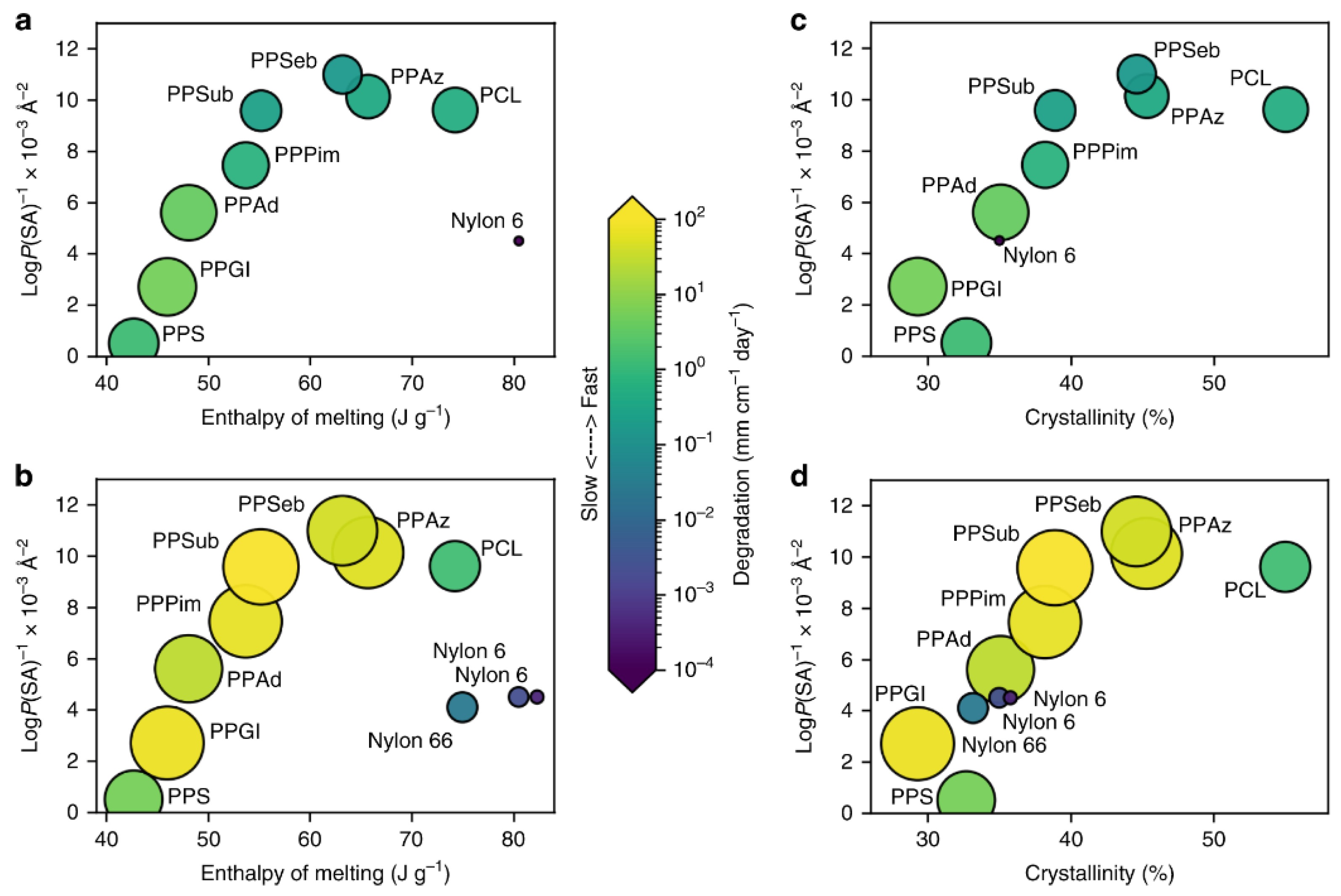
Figure 4. The influence of crystallinity and hydrophobicity on degradation [17]. The computational LogP(SA)−1 values are plotted versus the enthalpy of melting for abiotic hydrolysis (a), the enthalpy of melting for biotic processes (b), the % crystallinity for abiotic hydrolysis (c), the % crystallinity for biotic processes (d).The size of circles and colour is equivalent to surface erosion (in mg cm−2 day−1) in artificial seawater.
In their study, Yamawaki et al. performed virtual experiments for compost degradable polymers. As stated, no efficient system has yet been developed for practical use that considers multiple decomposition factors. Yamawaki et al. developed a prediction model for the degree of degradation, so as to investigate the degradation factors based on analytical data and experimental conditions [29]. This involved creating a predictive model using machine learning on a data set. The molecular weight received by GPC was the objective variable; the explanatory variables were the moisture content in a compost environment, the degradation time, the degree of crystallinity before the experiment and the NMR spectra. A decomposition degree predictive model was developed by considering the weight loss ratio as the objective variable. Different machine learning algorithms have compared the predictive accuracy of the predictive models. Furthermore, the NMR spectra have been compressed dimensionally using PCA (Principal Component Analysis). Explanatory variables were taken from the NMR data (crystallinity as analytical data and moisture content in the compost environment as experimental conditions). Figure 5 shows as a summary the concept of real and virtual degradable experiments that have been used.
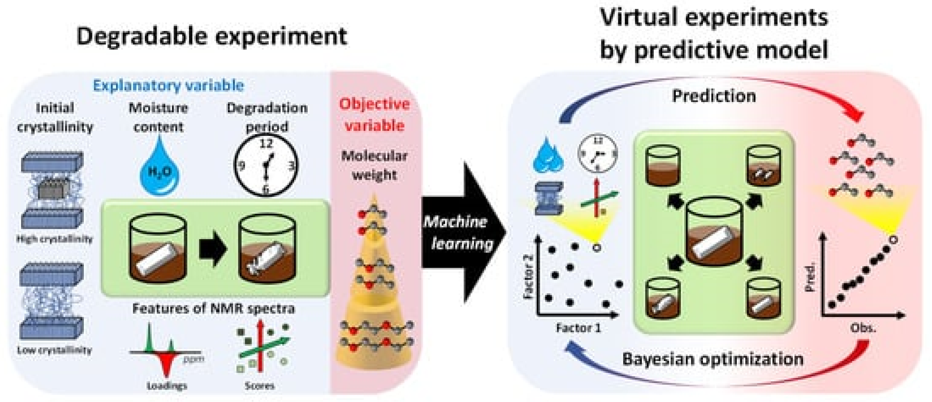
Figure 5. Real and virtual degradable experiments according to the study of Yamawaki et al. [29].
Decomposition experiments were conducted to achieve the ideal experimental conditions and different analytical data values (see Figure 5 left). The optimal degree of decomposition, different analytical values and experimental conditions were investigated by virtual experiments in combination with a predictive model and a Bayesian optimisation method (see Figure 5 right). Statistical variables were used to confirm the good accuracy of this predictive model. However, additional experimental conditions such as temperature and pH could lead to a more accurate predictive model [29].
2.3. Laboratory vs. Field Experiments: Outlook
Lott et al. recently investigated the performance of biodegradable plastic materials under marine-environment conditions. Biodegradation lab tests were compared with field tests. Furthermore, statistical modelling has been used to predict the half-life for the investigated materials under different environmental conditions [33]. The results have shown high variability in the biodegradation rate of biodegradable plastics under marine conditions, and the specific half-life times differed by different orders of magnitude ranging from weeks to years. Earlier, Albertsson and Karlsson, for instance, investigated PE photo-degradation in a so-called inert system in a 10-year experiment. They demonstrated that the PE degradation rate can be characterized by three different steps [34]. The biodegradation exhibits a complex phenomenon. It is still challenging to realize nature-like experiments in the laboratory. Many parameters must be taken into consideration. Each biodegradation stage needs an adapted estimation technique [18]. Biodegradation tests under laboratory conditions could lead to an overestimation of the biodegradation level regarding biodegradable plastics. Therefore, test standards should be developed for biodegradation to reduce the gaps between natural biodegradation compared to investigations carried out in the lab [35]. It has been shown previously in a 1000-h accelerated ageing test simulating outdoor conditions that biodegradable gillnets degraded faster than the nylon, which was used as a reference gillnet [36]. Based on these lab experiments, well-tailored biodegradable polymers and PA for fishing nets (gillnets) will be investigated in a long-term trial. Different laboratory tests and field trials will be carried out to ensure that the results represent the environmental factors prevailing in other countries [37]. Additionally, statistical models and data-driven techniques, and importantly, the investigation of mechanical forces on the rate of degradation, which needs further research, will help better understand the degradation behaviour of polymers in the sea and under composting conditions in the future.
References
- Echtermeyer, A.T.; Gagani, A.; Krauklis, A.; Mazan, T. Multiscale Modelling of Environmental Degradation—First Steps. In Durability of Composites in a Marine Environment 2. Solid Mechanics and Its Applications; Davies, P., Rajapakse, Y., Eds.; Springer: Berlin/Heidelberg, Germany, 2018; pp. 135–149.
- McGeorge, D.; Echtermeyer, A.; Leong, K.; Melve, B.; Robinson, M.; Fischer, K. Repair of floating offshore units using bonded fibre composite materials. Compos. Part A Appl. Sci. Manuf. 2009, 40, 1364–1380.
- Krauklis, A.E. Environmental Durability of Composite Materials: Analytical Modelling Toolbox. In Proceedings of the Aachen Reinforced, Symposium, Aachen, Germany, 11–13 May 2021.
- Siemens; Munich, Germany. Siemens case study. Personal communication, 2021.
- Lee, H.-S.; Rhee, S.Y.; Yoon, J.-H.; Yoo, J.-T.; Min, K.J. Establishment of Aerospace Composite Materials Data Center for Qualification. Compos. Res. 2015, 28, 402–407.
- Schafrik, R. Technology Transition in Aerospace Industry. In Proceedings of the Workshop on Accelerating Technology Transition, National Research Council, Washington, DC, USA, November 2003.
- Hagnell, M.; Kumaraswamy, S.; Nyman, T.; Åkermo, M. From aviation to automotive—A study on material selection and its implication on cost and weight efficient structural composite and sandwich designs. Heliyon 2020, 6, e03716.
- Offshore Energy. DNV GL: Two New JIPs Have Potential to Save Over $10M in Costs. Available online: https://www.offshore-energy.biz/dnv-gl-two-new-jips-have-potential-to-save-over-10m-in-costs/ (accessed on 10 November 2021).
- Bortolotti, P.; Berry, D.S.; Murray, R.; Gaertner, E.; Jenne, D.S.; Damiani, R.R.; EBarter, G.; Dykes, K.L. A Detailed Wind Turbine Blade Cost Model; Technical Report for National Renewable Energy Laboratory: Golden, CO, USA, 2019.
- Krauklis, A.E. Environmental Aging of Constituent Materials in Fiber-Reinforced Polymer Composites. Ph.D. Thesis, Norwegian University of Science and Technology, Trondheim, Norway, 2019.
- Lackner, M. Bioplastics. In Kirk-Othmer Encyclopedia of Chemical Technology; Wiley: Hoboken, NJ, USA, 2015.
- Chiellini, E.; Solaro, R. Biodegradable Polymeric Materials. Adv. Mater. 1996, 8, 305–313.
- Ghosh, K.; Jones, B.H. Roadmap to Biodegradable Plastics—Current State and Research Needs. ACS Sustain. Chem. Eng. 2021, 9, 6170–6187.
- Wang, G.-X.; Huang, D.; Ji, J.-H.; Völker, C.; Wurm, F.R. Seawater-Degradable Polymers—Fighting the Marine Plastic Pollution. Adv. Sci. 2020, 8, 2001121.
- Laycock, B.; Nikolić, M.; Colwell, J.M.; Gauthier, E.; Halley, P.; Bottle, S.; George, G. Lifetime prediction of biodegradable polymers. Prog. Polym. Sci. 2017, 71, 144–189.
- Rittié, L.; Perbal, B. Enzymes used in molecular biology: A useful guide. J. Cell Commun. Signal. 2008, 2, 25–45.
- Min, K.; Cuiffi, J.D.; Mathers, R.T. Ranking environmental degradation trends of plastic marine debris based on physical properties and molecular structure. Nat. Commun. 2020, 11, 1–11.
- Lucas, N.; Bienaime, C.; Belloy, C.; Queneudec, M.; Silvestre, F.; Nava-Saucedo, J.-E. Polymer biodegradation: Mechanisms and estimation techniques—A review. Chemosphere 2008, 73, 429–442.
- Gonzalez-Fernandez, C.; Sialve, B.; Molinuevo-Salces, B. Anaerobic digestion of microalgal biomass: Challenges, opportunities, and research needs. Bioresour. Technol. 2015, 198, 896–906.
- Mueller, R.-J. Biological degradation of synthetic polyesters—Enzymes as potential catalysts for polyester recycling. Process Biochem. 2006, 41, 2124–2128.
- Filiciotto, L.; Rothenberg, G. Biodegradable Plastics: Standards, Policies, and Impacts. ChemSusChem 2020, 14, 56–72.
- Krasowska, A.; Sigler, K. How microorganisms use hydrophobicity and what does this mean for human needs? Front. Cell. Infect. Microbiol. 2014, 4, 112.
- Webb, H.K.; Arnott, J.; Crawford, R.J.; Ivanova, E.P. Plastic Degradation and Its Environmental Implications with Special Reference to Poly(ethylene terephthalate). Polymers 2013, 5, 1–18.
- Dharmaratne, N.U.; Jouaneh, T.M.M.; Kiesewetter, M.K.; Mathers, R.T. Quantitative Measurements of Polymer Hydrophobicity Based on Functional Group Identity and Oligomer Length. Macromolecules 2018, 51, 8461–8468.
- Ben Halima, N. Poly(vinyl alcohol): Review of its promising applications and insights into biodegradation. RSC Adv. 2016, 6, 39823–39832.
- Avery-Gomm, S.; O’Hara, P.D.; Kleine, L.; Bowes, V.; Wilson, L.K.; Barry, K.L. Northern fulmars as biological monitors of trends of plastic pollution in the eastern North Pacific. Mar. Pollut. Bull. 2012, 64, 1776–1781.
- Erni-Cassola, G.; Zadjelovic, V.; Gibson, M.I.; Christie-Oleza, J.A. Distribution of plastic polymer types in the marine environment; a metaanalysis. J. Hazard. Mat. 2019, 369, 691–698.
- Haider, T.P.; Völker, C.; Kramm, J.; Landfester, K.; Wurm, F.R. Plastics of the Future? The Impact of Biodegradable Polymers on the Environment and on Society. Angew. Chem. Int. Ed. 2018, 58, 50–62.
- Yamawaki, R.; Tei, A.; Ito, K.; Kikuchi, J. Decomposition Factor Analysis Based on Virtual Experiments throughout Bayesian Optimization for Compost-Degradable Polymers. Appl. Sci. 2021, 11, 2820.
- Ollier, R.P.; Casado, U.; Nicolini, A.T.; Alvarez, V.A.; Pérez, C.J.; Ludueña, L.N. Improved creep performance of melt-extruded polycaprolactone/organo-bentonite nanocomposites. J. Appl. Polym. Sci. 2021, 138, 50961.
- Nanni, A.; Messori, M. Effect of the wine lees wastes as cost-advantage and natural fillers on the thermal and mechanical properties of poly(3-hydroxybutyrate-co-hydroxyhexanoate) (PHBH) and poly(3-hydroxybutyrate-co-hydroxyvalerate) (PHBV). J. Appl. Polym. Sci. 2020, 137, 48869.
- Amiri, A.; Yu, A.; Webster, D.; Ulven, C. Bio-Based Resin Reinforced with Flax Fiber as Thermorheologically Complex Materials. Polymers 2016, 8, 153.
- Lott, C.; Eich, A.; Makarow, D.; Unger, B.; van Eekert, M.; Schuman, E.; Reinach, M.S.; Lasut, M.T.; Weber, M. Half-Life of Biodegradable Plastics in the Marine Environment Depends on Material, Habitat, and Climate Zone. Front. Mar. Sci. 2021, 8, 426.
- Albertsson, A.-C.; Karlsson, S. The three stages in degradation of polymers—Polyethylene as a model substance. J. Appl. Polym. Sci. 1988, 35, 1289–1302.
- Choe, S.; Kim, Y.; Won, Y.; Myung, J. Bridging Three Gaps in Biodegradable Plastics: Misconceptions and Truths About Biodegradation. Front. Chem. 2021, 9, 671750.
- Grimaldo, E.; Herrmann, B.; Jacques, N.; Kubowicz, S.; Cerbule, K.; Su, B.; Larsen, R.; Vollstad, J. The effect of long-term use on the catch efficiency of biodegradable gillnets. Mar. Pollut. Bull. 2020, 161, 111823.
- Karl, C.W.; Grimaldo, E.; Benjaminsen, C. Combating Marine Waste and Ghost Fishing with New Materials. Norwegian Science Tech News, May 2021. Available online: https://norwegianscitechnews.com/2021/06/combating-marine-waste-and-ghost-fishing-with-new-materials/(accessed on 28 September 2021).
More
Information
Subjects:
Polymer Science
Contributor
MDPI registered users' name will be linked to their SciProfiles pages. To register with us, please refer to https://encyclopedia.pub/register
:
View Times:
2.4K
Revisions:
2 times
(View History)
Update Date:
15 Mar 2022
Table of Contents


Notice
You are not a member of the advisory board for this topic. If you want to update advisory board member profile, please contact office@encyclopedia.pub.
OK
Confirm
Only members of the Encyclopedia advisory board for this topic are allowed to note entries. Would you like to become an advisory board member of the Encyclopedia?
Yes
No
${ textCharacter }/${ maxCharacter }
Submit
Cancel
Back
Comments
${ item }
|
${ item.createdUser.fullName }
${ item.createdAt }
${ item.vote }
${ item.reply }
Delete
${ reply.createdUser.fullName }
${ reply.createdAt }
${ reply.vote }
Delete
There is no reply to this comment~
${ item.replyTextCharacter }/${ item.replyMaxCharacter }
Submit
Cancel
More
No more~
There is no comment~
${ textCharacter }/${ maxCharacter }
Submit
Cancel
${ selectedItem.replyTextCharacter }/${ selectedItem.replyMaxCharacter }
Submit
Cancel
Confirm
Are you sure to Delete?
Yes
No