 +1 credit
| Version | Summary | Created by | Modification | Content Size | Created at | Operation |
|---|---|---|---|---|---|---|
| 1 | Manje Gowda | + 3586 word(s) | 3586 | 2020-09-09 08:37:49 | | | |
| 2 | Rita Xu | -1153 word(s) | 2433 | 2020-09-09 11:54:57 | | |
Video Upload Options
To dissect the genetic architecture of Common rust (CR) resistance caused by Puccina sorghi in maize, we applied association mapping, in conjunction with linkage mapping, joint linkage association mapping (JLAM), and genomic prediction (GP) was conducted on an association-mapping panel and five F3 biparental populations using genotyping-by-sequencing (GBS) single-nucleotide polymorphisms (SNPs). Genome-wide association study (GWAS) analyses revealed 14 significant marker-trait associations which individually explained 6–10% of the total phenotypic variances. Individual population-based linkage analysis revealed 26 QTLs associated with CR resistance and together explained 14–40% of the total phenotypic variances. JLAM for the 921 F3 families from five populations detected 18 QTLs distributed in all chromosomes except on chromosome 8. These QTLs individually explained 0.3 to 3.1% and together explained 45% of the total phenotypic variance. Among the 18 QTL detected through JLAM, six QTLs, qCR1-78, qCR1-227, qCR3-172, qCR3-186, qCR4-171, and qCR7-137 were also detected in linkage mapping. GP within population revealed low to moderate correlations with a range from 0.19 to 0.51. Prediction correlation was high with r = 0.78 for combined analysis of the five F3 populations. Prediction of biparental populations by using association panel as training set reveals positive correlations ranging from 0.05 to 0.22, which encourages to develop an independent but related population as a training set which can be used to predict diverse but related populations. The findings of this study provide valuable information on understanding the genetic basis of CR resistance and the obtained information can be used for developing functional molecular markers for marker-assisted selection and for implementing GP to improve CR resistance in tropical maize.
1. Introduction
Common rust (hereafter CR) caused by Puccina sorghi is one of the most destructive foliar diseases in maize-growing regions predominantly in humid areas and has been reported to cause 12 to 61% yield losses in a favorable environments [1][2]. These yield losses are subject to leaf area infected and host growth stages whereby the former has been estimated to cause about 3–8% yield loss for each 10% of the total leaf area affected [3]. Quantitative resistance is due to partial resistance or adult plant resistance [4]. Numerous studies have suggested that older and mature tissues have more resistance to CR than younger soft tissues [4][5][6].
Past efforts to control CR through conventional means have been largely unsuccessful and also affected by unpredictable weather, and the use of fungicides leads to environmental effects and increased production costs [7]. Host-plant resistance has been identified as the most reliable and economically viable option among several available options to alleviate plant diseases [7][8]. In the case of CR, researchers have identified both qualitative and quantitative resistance [9][10]. Resistance through R genes has been identified more than 25 dominant race-specific (Rp) genes in chromosomes (chr) 3, 4, and 10 [9][11], which mediate the recognition of the pathogen and trigger a hypersensitive reaction to prevent further spread of the pathogen [12]. However, novel P. sorghi races can overcome the qualitative resistance in some genotypes and this requires a continuous search for sources of stable and durable resistance (quantitative) in order to manage the disease. Identifying resistant germplasm to CR and incorporation of resistant genes or genomic regions to elite lines and commercial hybrids has the potential to increase yields with lower production costs [13].
Genetic mapping through linkage analyses and genome-wide association study (GWAS) have been used in many studies in plant breeding [12][14][15][16][17][18][19][20][21][22][23][24][25][26]. The two approaches exploit the recombination’s ability to break up the genome into fragments that can be correlated with phenotypic variation but differ with the type of control they have on the recombination [27]. Linkage mapping in plants utilizes biparental crosses and, thus, is a closed controlled system. This further limits the number of recombinations that can sufficiently shuffle the genome into small fragments and results into QTLs localized in large chromosomal regions [28]. On the other hand, GWAS uses natural populations that mimic historical recombinations and provide a higher resolution compared to linkage mapping [25]. This approach, however, has no control over relatedness and is prone to spurious associations. Accounting for population structure and kinship relatedness in a mixed model has been the most effective method of reducing false associations in GWAS [29]. Quantitative resistance for CR, a more durable approach, has also been exploited in a few studies through quantitative trait loci (QTL) analysis and genome-wide association studies (GWAS). A total of 41 QTLs have been identified conferring resistance to CR across all maize chromosomes in four separate studies utilizing different maize germplasm [7][10][13][30]. One study by Olukolu et al. [12], carried out GWAS and identified three marker trait associations (MTAs) in chr 2, 3, and 8 using 274 diverse inbred lines and 246,497 SNPs. Another study combined linkage and association mapping on 296 tropical maize inbreds and identified 25 QTLs on chr 1, 3, 5, 6, 8, and 10 associated with CR resistance [31]. These markers and candidate genes were directly or indirectly involved with plant disease responses [12][31].
In cases where the phenotype is strongly correlated with relatedness, population mapping even with the use of mixed models can be severely under powered [27]. Joint linkage association mapping (JLAM) has the potential to overcome the downsides of the both linkage mapping and association mapping approaches whereby one compliments the other. Association mapping will increase the mapping resolution power while linkage mapping will account for relatedness in cases where Q + K explains most of the phenotypic variance. To our knowledge, no study has been reported utilizing JLAM to identify QTLs conferring resistance to CR in maize.
Another promising genomic tool is the genomic prediction (GP) which has been applied successfully in many plant breeding programs [32][33]. Previous reports indicated the potential of GP to increase genetic gain and reduce the time taken in breeding programs significantly [33]. GP utilizes genome-wide markers to estimate the effects of all loci and computes a genomic estimated breeding value (GEBVs) [34]. Unlike genetic mapping, GP does not identify significant marker-trait associations (MTAs) first but goes ahead to use all markers available to estimate their effects thus providing a powerful approach to account for any effects that might have been missed by genetic mapping.
2. Results
Comparable disease pressure was observed in each environment as indicated by significant genotypic variance at each environment for each population (Table S1). Further, significant (p < 0.05) Pearson correlations were also observed among phenotypic values determined at different environments for each population (Table S2). This suggested that there was enough CR disease pressure in each environment. Cross-environment analyses revealed normal distributions of CR disease severity (score 1–9) in the F3 populations and IMAS association panel, ranging from high resistance to moderate susceptibility with scores ranging from 2.0 to 6.0 and with average means ranging from 3.4 to 4.1 for different populations (Table 1 and Figure 1). Analysis of variance for the biparental populations and the association panel showed significant genotypic and genotype x environment (GXE) variances except for GXE of Pop1 and Pop4 (Table 1). Heritability (h2) estimates were moderate with range of 0.37–0.45 for the individual F3 populations, 0.45 across the F3 populations and 0.65 for the IMAS panel.
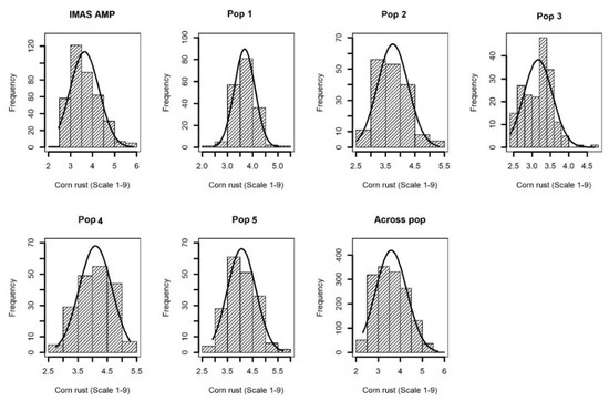
Figure 1. Phenotypic distribution for corn rust or common rust severity in the IMAS association panel, five F3 populations and across F3 populations.
Table 1. Means, ranges, and components of variance for Common rust in an IMAS association panel, F3 populations and across F3 populations.
| Population | Mean (Range) | σ2G | σ2GxE | σ2e | h2 |
|---|---|---|---|---|---|
| IMAS AMP | 3.80 (2.40–5.90) | 0.07 * | 0.03 * | 0.13 | 0.68 |
| CZL0618 × LaPostaSeqC7-F71-1-2-1-1B–Pop1 | 3.61 (2.00–5.50) | 0.024 * | 0.01 | 0.10 | 0.44 |
| CZL074 × LaPostaSeqC7-F103-1-2-1-1B–Pop2 | 3.70 (2.50–5.30) | 0.02 * | 0.02 * | 0.12 | 0.43 |
| CZL00009 × CZL99017–Pop3 | 3.42 (2.32–5.00) | 0.03 * | 0.02 * | 0.11 | 0.45 |
| CML505 × CZL99017–Pop4 | 4.10 (2.76–5.14) | 0.01 * | 0.01 | 0.12 | 0.37 |
| CZL0723 × CZL0724–Pop5 | 4.02 (2.51–6.02) | 0.03 * | 0.02 * | 0.16 | 0.38 |
| Across five populations | 3.85 (2.02–6.00) | 0.04 * | 0.10 * | 0.15 | 0.45 |
An IMAS association mapping panel was earlier used to study the maize lethal necrosis resistance [20], where the population structure was reported in detail. In the IMAS panel, a rapid linkage disequilibrium (LD) decay across physical distance in kb was reported (Figure 2). At LD cut-off points of r2 = 0.1, the average physical distance was 14.97 kilo base pairs. GWAS was performed using a mixed linear model by integrating population structure (PCA) and family relatedness (kinship) within the IMAS panel using 337,110 high quality SNPs. GWAS for CR identified 14 significant marker-trait associations (MTA, significant threshold p < 9 × 10⁻⁶). These SNPs were found across all chromosomes except on chr 6, 7, and 8 (Table 2 and Figure 3). The distribution of SNPs across chromosomes and their level of significance for CR are shown in a Manhattan plot (Figure 3A). To test the ability of the model used, a quantile-quantile plot of the observed-log p-value vs. the expected-log p-value was plotted. As shown in Figure 3B, the population structure was controlled well by the mixed linear model (Figure 3). In terms of the percentage of phenotypic variance explained (PVE), the SNPs identified from GWAS individually explained 6–10% (Table 2). SNP S5_51353429 had the largest significant MTA while S3_21856582 explained the most phenotypic variance. Candidate genes were selected around the significant SNPs and identify the putative function of these genes. Six candidate genes were identified in the significant SNP sites or adjacent to these sites (Table 2). We identified two candidate genes each on chromosomes 2, 5, and 10.
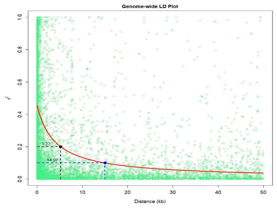
Figure 2. Linkage disequilibrium (LD) plot representing the average genome-wide LD decay in the panels with genome-wide markers. The values on the Y-axis represents the squared correlation coefficient r2 and the X-axis represents the physical distance in (kb).

Figure 3. (A) Manhattan and q–q plots for the GWAS of common rust for the IMAS association mapping panel. The dashed horizontal line of the Manhattan plot depicts the significance threshold (p < 9 × 10⁻⁶). The X-axis indicates the SNP location along the 10 chromosomes, with chromosomes separated by different colors. (B) The red line on the q–q plot indicates a line of best fit with trait significance determined by a plot of expected-log10 (p) against observed-log10 (p).
Table 2. Chromosomal position and SNPs significantly associated with Common rust disease severity (DS) detected by SNP-based GWAS in the IMAS association mapping panel.
| SNP a | Chr | MLM-P Value | R2 (%) | MAF | Allele | Putative Candidate Genes | Predicted Function of Candidate Gene |
|---|---|---|---|---|---|---|---|
| S1_12663024 | 1 | 4.86 × 10⁻⁶ | 7.00 | 0.14 | A/G | GRMZM2G480386 | uncharacterized |
| S1_41433126 | 1 | 4.69 × 10⁻⁶ | 7.88 | 0.05 | G/A | GRMZM5G886521 | uncharacterized |
| S1_220067760 | 1 | 5.86 × 10⁻⁷ | 7.80 | 0.46 | C/T | GRMZM2G564469 | uncharacterized |
| S2_16361185 | 2 | 5.23 × 10⁻⁶ | 7.70 | 0.08 | C/T | GRMZM2G086484 | Pleckstrin homology (PH) domain superfamily protein |
| S2_222274747 | 2 | 7.65 × 10⁻⁶ | 7.10 | 0.05 | C/T | GRMZM2G009188 | 11-beta-hydroxysteroid dehydrogenase 1B |
| S3_21856582 | 3 | 3.84 × 10⁻⁶ | 9.54 | 0.42 | A/C | GRMZM2G395983 | uncharacterized |
| S3_34683394 | 3 | 4.83 × 10⁻⁶ | 9.02 | 0.35 | A/G | GRMZM5G881063 | uncharacterized |
| S3_147013779 | 3 | 3.89 × 10⁻⁶ | 7.70 | 0.17 | G/C | GRMZM2G060540 | uncharacterized |
| S4_130478096 | 4 | 6.72 × 10⁻⁶ | 6.93 | 0.12 | A/T | GRMZM5G833902 | uncharacterized |
| S5_10087070 | 5 | 8.02 × 10⁻⁶ | 6.25 | 0.06 | A/G | GRMZM2G181002 | Phosphotransferases, Serine or threonine-specific kinase subfamily |
| S5_10089138 | 5 | 4.39 × 10⁻⁶ | 6.56 | 0.07 | T/C | GRMZM2G181002 | |
| S5_51353429 | 5 | 9.05 × 10⁻⁶ | 7.40 | 0.19 | G/A | GRMZM2G457211 | uncharacterized |
| S10_134585613 | 10 | 3.68 × 10⁻⁶ | 6.65 | 0.12 | C/T | GRMZM2G322582 | ATP binding protein |
| S10_134831452 | 10 | 4.78 × 10⁻⁷ | 8.22 | 0.14 | A/G | GRMZM2G181030 | MYB-related transcription factor family that regulates hypocotyl growth by regulating free auxin levels in a time-of-day specific manner (RVE1) |
Linkage map for each of the five populations was constructed. For each population, the number of progenies or families, markers, map lengths, and average genetic distances between the markers are presented in Table S3. Detection of QTL in the F3 populations revealed seven QTLs in pop1, nine QTL in pop2, four QTL in pop3, five QTL in pop4 and one QTL in pop5, distributed on all chromosomes except chromosome 10 (Table 3). In pop1, QTLs individually explained 3–7% of phenotypic variance, in pop2, individual QTL explained 2–11% of total variation. In pop3, each QTL explained 5–9% of variation, whereas the range was 3–20% in pop4 and 17% in pop5. The total variance explained by each population ranged from 14 to 40%. Comparison of QTL detected among five populations revealed that QTL qCR1-78 was detected in both pop1 and pop5 on chromosome 1. Another QTL qCR3-151 detected in pop2 was within the confidence interval of the QTL qCR3-113 detected in pop1 (Table 3). QTL qCR9-117 detected in pop3 overlapped with QTL qCR9-118 observed in pop2.
Table 3. Detection of QTL associated with resistance to Common rust, their physical positions and genetic effects in five F3 populations.
| QTL Name | Chr | Position (cM) | LOD | PVE (%) | Add | Dom | Total PVE (%) | Left Marker | Right Marker |
|---|---|---|---|---|---|---|---|---|---|
| CZL0618 × LaPostaSeqC7-F71-1-2-1-1B–Pop1 | |||||||||
| qCR1-78 | 1 | 551 | 4.41 | 3.32 | −0.20 | −0.08 | 14.95 | S1_77801418 | S1_80167797 |
| qCR1-290 | 1 | 799 | 2.82 | 3.59 | 0.18 | −0.13 | S1_290957469 | S1_285979058 | |
| qCR2-198 | 2 | 187 | 3.17 | 6.70 | −0.34 | −0.53 | S2_198394488 | S2_230388748 | |
| qCR3-113 | 3 | 307 | 2.85 | 6.50 | 0.26 | −0.24 | S3_224567900 | S3_113425715 | |
| qCR6-38 | 6 | 194 | 2.79 | 3.62 | 0.21 | −0.01 | S6_37902339 | S6_63537451 | |
| qCR6-63 | 6 | 197 | 4.51 | 3.27 | −0.21 | −0.02 | S6_63537451 | S6_65299800 | |
| qCR6-146 | 6 | 446 | 3.09 | 7.03 | 0.30 | −0.42 | S6_147225115 | S6_146382028 | |
| CZL074 × LaPostaSeqC7-F103-1-2-1-1B–Pop2 | |||||||||
| qCR2-137 | 2 | 414 | 2.54 | 2.38 | 0.00 | 0.18 | 39.5 | S2_158674609 | S2_136562142 |
| qCR3-8 | 3 | 262 | 3.33 | 2.97 | 0.63 | 0.52 | S3_8300745 | S3_8888914 | |
| qCR3-151 | 3 | 405 | 6.56 | 6.28 | 0.17 | −0.14 | S3_150831482 | S3_166811360 | |
| qCR4-198 | 4 | 351 | 2.58 | 5.64 | −0.19 | −0.05 | S4_197820294 | S4_200964285 | |
| qCR4-198 | 4 | 354 | 5.77 | 8.85 | 0.24 | 0.01 | S4_200964285 | S4_198430250 | |
| qCR5-51 | 5 | 374 | 2.93 | 3.7 | −0.17 | 0.27 | S5_186678634 | S5_51355494 | |
| qCR8-123 | 8 | 165 | 4.69 | 6.23 | 0.20 | 0.00 | S8_130213071 | S8_123469991 | |
| qCR9-118 | 9 | 291 | 2.55 | 8.46 | −0.23 | 0.03 | S9_120748383 | S9_118065757 | |
| qCR9-12 | 9 | 359 | 5.63 | 10.95 | −0.28 | −0.03 | S9_12599819 | S9_11929364 | |
| CZL00009 × CZL99017–Pop3 | |||||||||
| qCR1-18 | 1 | 394 | 3 | 5.21 | −0.13 | −0.08 | 12.99 | S1_19328973 | S1_17679542 |
| qCR1-172 | 1 | 501 | 2.81 | 6.09 | 0.67 | −0.6 | S1_196052894 | S1_171534815 | |
| qCR2-16 | 2 | 93 | 3.61 | 5.84 | 0.7 | −0.47 | S2_16401968 | S2_181538947 | |
| qCR9-117 | 9 | 300 | 4.31 | 8.35 | −0.18 | −0.04 | S9_122035011 | S9_116948078 | |
| CML505 × CZL99017–Pop4 | |||||||||
| qCR1-139 | 1 | 182 | 3.87 | 20.16 | 0.32 | 0.67 | 23.89 | S1_139463362 | S1_227241027 |
| qCR4-171 | 4 | 239 | 4.83 | 5.55 | −0.23 | 0.01 | S4_171215058 | S4_173802342 | |
| qCR7-137 | 7 | 87 | 9.79 | 11.01 | −0.34 | 0.22 | S7_140894965 | S7_137169719 | |
| qCR9-47 | 9 | 410 | 3.03 | 2.79 | 0.11 | −0.24 | S9_47064183 | S9_58143264 | |
| qCR9-90 | 9 | 432 | 3.18 | 3 | −0.13 | −0.2 | S9_90366846 | S9_97737243 | |
| CZL0723 × CZL0724–Pop5 | |||||||||
| qCR1-77 | 1 | 89 | 6.52 | 17.39 | 0.29 | −0.09 | 14.28 | S1_73375502 | S1_77145631 |
All five F3 populations and IMAS panel was plotted by using first three principal components, which together contributed for 27.5% of the variation. PCA plot showed clear clustering of the five F3 populations and IMAS panel into five clusters as shown in Figure 4. PCA distribution suggests pop 1 and pop 2 are more related to the IMAS panel compared to pop 3, 4, and 5. Joint linkage association mapping across five F3 populations constituted 921 families, identified eighteen QTLs distributed in all chromosomes except on chromosome 8 (Table 4). These QTLs individually explained 0.3 to 3.1% and together explained 45% of the total phenotypic variance. Among the 18 QTL detected through JLAM, six QTLs, qCR1-78, qCR1-227, qCR3-172, qCR3-186, qCR4-171, and qCR7-137 were also detected in individual population-based linkage mapping (Table 3). Out of these 18 QTLs, one QTL on chromosome 7 (qCR7-10) followed by QTL on chromosome 1 (qCR1-78) were strongly associated with CR disease severity in terms of p values.
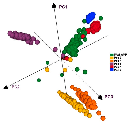
Figure 4. PCA analyses of five F3 populations and the IMAS panel based on GBS markers.
Table 4. Analysis of trait-associated markers, allele substitution (α) effects, and the total phenotypic variance (R2) of the joint linkage association mapping based on combined five F3 populations.
| Marker | QTL_Name a | Chrom | Pos | α-effect | p Value | PVE (%) | PG |
|---|---|---|---|---|---|---|---|
| S1_77801418 | qCR1_78 | 1 | 77.80 | 0.16 | 1.34 × 10⁻¹² | 2.9 | 7.2 |
| S1_227241027 | qCR1_227 | 1 | 227.24 | 0.17 | 3.75 × 10⁻⁷ | 1.5 | 3.8 |
| S2_20589802 | qCR2_20 | 2 | 205.90 | 0.11 | 1.51 × 10⁻³ | 0.6 | 1.5 |
| S3_172332492 | qCR3_172 | 3 | 172.33 | −0.06 | 1.50 × 10⁻² | 0.3 | 0.7 |
| S3_186725598 | qCR3_186 | 3 | 186.73 | 0.10 | 9.88 × 10⁻³ | 0.4 | 1 |
| S4_828312 | qCR4_1 | 4 | 0.83 | −0.19 | 6.02 × 10⁻¹⁰ | 2.2 | 5.5 |
| S4_5238963 | qCR4_5 | 4 | 5.24 | 0.12 | 7.45 × 10⁻⁸ | 1.6 | 4 |
| S4_171215058 | qCR4_171 | 4 | 171.22 | −0.05 | 3.79 × 10⁻² | 0.2 | 0.5 |
| S5_2363546 | qCR5_2 | 5 | 2.36 | −0.06 | 2.03 × 10⁻² | 0.3 | 0.7 |
| S6_32969273 | qCR6_32 | 6 | 32.97 | 0.10 | 4.49 × 10⁻⁵ | 0.9 | 2.2 |
| S6_144280146 | qCR6_144 | 6 | 144.28 | 0.06 | 2.57 × 10⁻² | 0.3 | 0.7 |
| S6_154981658 | qCR6_155 | 6 | 154.98 | −0.19 | 8.37 × 10⁻⁴ | 0.6 | 1.5 |
| S7_10651847 | qCR7_10 | 7 | 10.65 | −0.28 | 1.78 × 10⁻¹³ | 3.1 | 7.8 |
| S7_13389227 | qCR7_13 | 7 | 133.89 | 0.20 | 3.25 × 10⁻¹¹ | 2.5 | 6.2 |
| S7_137335046 | qCR7_137 | 7 | 137.34 | −0.14 | 3.26 × 10⁻⁹ | 2 | 5 |
| S9_134919722 | qCR9_135 | 9 | 134.92 | −0.14 | 5.08 × 10⁻⁵ | 0.9 | 2.2 |
| S10_132612571 | qCR10_132 | 10 | 132.61 | −0.15 | 2.76 × 10⁻⁹ | 2 | 5 |
| S10_133744261 | qCR10_133 | 10 | 133.74 | −0.09 | 1.79 × 10⁻³ | 0.5 | 1.2 |
We used the RR-BLUP model to predict the lines performance within each population. The prediction correlation was highest for pop4 (r = 0.51) followed by the IMAS panel (r = 0.46) and pop 2 (r = 0.46) and was low for pop3 with 0.19 (Figure 5A). However, the prediction through combined analysis of the five F3 populations reported high improvement in the prediction accuracy with 0.78 for CR (Figure 5A). Prediction of biparental populations by using IMAS panel as training population reveals the correlations of 0.15, 0.05, −0.14, 0.22 and 0.07 for pop1, pop2, pop3, pop4, and pop5, respectively (Figure 5B).
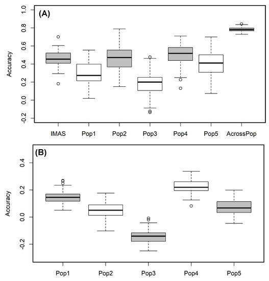
Figure 5. Genome-wide prediction correlations for CR resistance in bi-parental and IMAS AM panel based on two different scenarios. Scenario (A) estimation and prediction within IMAS AM panel and biparental populations and combined F3 populations; Scenario (B): prediction of each F3 population using IMAS AM panel as a training set with five-fold cross-validation.
References
- Dey, U.; Harlapur, S.I.; Dhutraj, D.N.; Suryawanshi, A.P.; Bhattacharjee, R. Integrated disease management strategy of common rust of maize incited by Puccinia sorghi Schw. Afr. J. Microbiol. Res. 2015, 9, 1345–1351.
- Dey, U.; Harlapur, S.I.; Dhutraj, D.N.; Suryawanshi, A.P.; Badgujar, S.L.; Jagtap, G.P.; Kuldhar, D.P. Spatiotemporal yield loss assessment in corn due to common rust caused by Puccinia sorghi Schw. African, J. Agric. Res. 2012, 7, 5265–5269.
- Crautam, P.; Stein, J. Induction of systemic acquired resistance to Puccinia sorghi in corn. Inter. J. Plant Pathol. 2011, 2, 43–50.
- Chandler, M.A.; Tracy, W.F. Vegetative phase change among sweet corn (Zea mays L.) hybrids varying for reaction to common rust (Puccinia sorghi Schw.). Plant Breed. 2007, 126, 569–573.
- Abedon, B.G.; Tracy, W.F. Corngrass 1 of maize (Zea mays L.) delays development of adult plant resistance to common rust (Puccinia sorghi Schw.) and European corn borer (Ostrinia nubilalis Hubner). J. Hered. 1996, 87, 219–223.
- Hurkman, M.M. Vegetative phase transition and response to disease in maize (Zea mays L.). Ph.D. Thesis, University of Wisconsin, Madison, WI, USA, 2003. Available online: https://elibrary.ru/item.asp?id=5282527 (accessed on 15 August, 2020).
- Danson, J.; Lagat, M.; Kimani, M.; Kuria, A. Quantitative trait loci (QTLs) for resistance to gray leaf spot and common rust diseases of maize. African, J. Biotechnol. 2008, 7, 3247–3254.
- Ayiga-Aluba, J.; Edemal, R.; Tusiime, G.; Asea, G.; Gibson, P. Response to two cycles of S1 recurrent selection for turcicum leave blight in an open pollinated maize variety population (Longe 5). Adv. Appl. Sci. Res. 2015, 6, 4–12.
- Delaney, D.E.; Webb, C.A.; Hulbert, S.H. A novel rust resistance gene in maize showing overdominance. Mol. plant-microbe Interact. 1998, 11, 242–245.
- Lübberstedt, T.; Klein, D.; Melchinger, A.E. Comparative quantitative trait loci mapping of partial resistance to Puccinia sorghi across four populations of European flint maize. Phytopathology 1998, 88, 1324–1329.
- Hooker, A.L. Corn and sorghum rusts. In Diseases, Distribution, Epidemiology, and Control; Elsevier: Amsterdam, Netherlands, 1985; pp. 207–236.
- Olukolu, B.A.; Tracy, W.F.; Wisser, R.; De Vries, B.; Balint-Kurti, P.J. A Genome-Wide Association Study for Partial Resistance to Maize Common Rust. Phytopathology 2016, 106, 745–751.
- Brown, A.F.; Juvik, J.A.; Pataky, J.K. Quantitative trait loci in sweet corn associated with partial resistance to Stewart’s wilt, northern corn leaf blight, and common rust. Phytopathology 2001, 91, 293–300.
- Kump, K.L.; Bradbury, P.J.; Wisser, R.J.; Buckler, E.S.; Belcher, A.R.; Oropeza-Rosas, M.A.; Zwonitzer, J.C.; Kresovich, S.; McMullen, M.D.; Ware, D. Genome-wide association study of quantitative resistance to southern leaf blight in the maize nested association mapping population. Nat. Genet. 2011, 43, 163.
- Zila, C.T.; Fernando Samayoa, L; Santiago, R.; Butrón, A.; Holland, J.B. A Genome-Wide Association Study Reveals Genes Associated with Fusarium Ear Rot Resistance in a Maize Core Diversity Panel. G3 (Bethesda). 2013, 3, 2095–2104.
- Laidò, G.; Marone, D.; Russo, M.A.; Colecchia, S.A.; Mastrangelo, A.M.; De Vita, P.; Papa, R. Linkage Disequilibrium and Genome-Wide Association Mapping in Tetraploid Wheat (Triticum turgidum L.). PLoS ONE 2014, 9, e95211.
- Ding, J.; Ali, F.; Chen, G.; Li, H.; Mahuku, G.; Yang, N.; Narro, L.; Magorokosho, C.; Makumbi, D.; Yan, J. Genome-wide association mapping reveals novel sources of resistance to northern corn leaf blight in maize. BMC Plant Biol. 2015, 15, 206.
- Gowda, M.; Das, B.; Makumbi, D.; Babu, R.; Semagn, K.; Mahuku, G.; Olsen, M.S.; Bright, J.M.; Beyene, Y.; Prasanna, B.M. Genome-wide association and genomic prediction of resistance to maize lethal necrosis disease in tropical maize germplasm. Theor. Appl. Genet. 2015, 128, 1957–1968.
- Cui, Z.; Luo, J.; Qi, C.; Ruan, Y.; Li, J.; Zhang, A.; Yang, X.; He, Y. Genome-wide association study (GWAS) reveals the genetic architecture of four husk traits in maize. BMC Genomics 2016, 17, 946.
- Gustafson, T.J.; de Leon, N.; Kaeppler, S.M.; Tracy, W.F. Genetic Analysis of Sugarcane mosaic virus Resistance in the Wisconsin Diversity Panel of Maize. Crop Sci. 2018, 58, 1853–1865.
- Liu, N.; Xue, Y.; Guo, Z.; Li, W.; Tang, J. Genome-Wide Association Study Identifies Candidate Genes for Starch Content Regulation in Maize Kernels. Front. Plant Sci. 2016, 7, 1046.
- Kuki, M.C.; Scapim, C.A.; Rossi, E.S.; Mangolin, C.A.; do Amaral Junior, A.T.; Pinto, R.J.B. Genome wide association study for gray leaf spot resistance in tropical maize core. PLoS ONE 2018, 13, e0199539.
- Chaikam, V.; Gowda, M.; Nair, S.; Melchinger, A.; Prasanna, B. Genome-wide association study to identify genomic regions influencing spontaneous fertility in maize haploids. Euphytica 2019, 215, 138.
- Nyaga, C.; Gowda, M.; Beyene, Y.; Muriithi, W.; Makumbi, D.; Olsen, M.; Suresh, L.M.; Bright, J.; Das, B.; Prasanna, B. Genome-Wide Analyses and Prediction of Resistance to MLN in Large Tropical Maize Germplasm. Genes 2019, 11, 16.
- Jaiswal, V.; Gupta, S.; Gahlaut, V.; Muthamilarasan, M.; Bandyopadhyay, T.; Ramchiary, N.; Prasad, M. Genome-Wide Association Study of Major Agronomic Traits in Foxtail Millet (Setaria italica L.) Using ddRAD Sequencing. Sci. Rep. 2019, 9, 5020.
- Sitonik, C.; Suresh, L.M.; Beyene, Y.; Olsen, M.S.; Makumbi, D.; Oliver, K.; Das, B.; Bright, J.M.; Mugo, S.; Crossa, J.; et al. Genetic architecture of maize chlorotic mottle virus and maize lethal necrosis through GWAS, linkage analysis and genomic prediction in tropical maize germplasm. Theor. Appl. Genet. 2019, 132, 2381-2399.
- Myles, S.; Peiffer, J.; Brown, P.J.; Ersoz, E.S.; Zhang, Z.; Costich, D.E.; Buckler, E.S. Association mapping: Critical considerations shift from genotyping to experimental design. Plant Cell 2009, 21, 2194–2202.
- Holland, J.B. Genetic architecture of complex traits in plants. Curr. Opin. Plant Biol. 2007, 10, 156–161.
- Kang, H.M.; Zaitlen, N.A.; Wade, C.M.; Kirby, A.; Heckerman, D.; Daly, M.J.; Eskin, E. Efficient control of population structure in model organism association mapping. Genetics 2008, 178, 1709–1723.
- Kerns, M.R.; Dudley, J.W.; Rufener, G.K. QTL for resistance to common rust and smut in maize. Maydica 1999, 44, 37–45.
- Zheng, H.; Chen, J.; Mu, C.; Makumbi, D.; Xu, Y.; Mahuku, G. Combined linkage and association mapping reveal QTL for host plant resistance to common rust (Puccinia sorghi) in tropical maize. BMC Plant Biol. 2018, 18, 310.
- Lorenz, A.J.; Chao, S.; Asoro, F.G.; Heffner, E.L.; Hayashi, T.; Iwata, H.; Smith, K.P.; Sorrells, M.E.; Jannink, J.L. Genomic Selection in Plant Breeding: Knowledge and Prospects. Adv. Agron. 2011, 110, 77–123.
- Crossa, J.; Pérez-Rodríguez, P.; Cuevas, J.; Montesinos-López, O.; Jarquín, D.; de los Campos, G.; Burgueño, J.; González-Camacho, J.M.; Pérez-Elizalde, S.; Beyene, Y.; et al. Genomic Selection in Plant Breeding: Methods, Models, and Perspectives. Trends Plant Sci. 2017, 22, 961–975.
- Massman, J.M.; Gordillo, A.; Lorenzana, R.E.; Bernardo, R. Genomewide predictions from maize single-cross data. Theor. Appl. Genet. 2013, 126, 13–22.

