Machine Learning Based Restaurant Sales Forecasting

Version	Summary	Created by	Modification	Content Size	Created at	Operation
1		Md Tamjidul Hoque	+ 2839 word(s)	2839	2022-02-08 03:34:18	\|
2	update layout	Amina Yu	+ 1401 word(s)	4240	2022-02-09 05:31:57	\| \|
3	update references and layout	Amina Yu	+ 1402 word(s)	4241	2022-02-09 06:29:56	\| \|
4	update Supplementary materials	Amina Yu	-1390 word(s)	2851	2022-02-10 07:50:35	\|

This entry is adapted from the peer-reviewed paper 10.3390/make4010006

A machine learning (ML) model is ideally trained using an optimal number of features and will capture fine details in the prediction task, such as holidays, without underperforming when the forecast window increases from one day to one week.

recurrent neural networks transformers forecasting restaurant sales prediction

1. Introduction

Small and medium-sized restaurants often have trouble forecasting sales due to a lack of data or funds for data analysis. The motivation for forecasting sales is that every restaurant has time-sensitive tasks which need to be completed. For example, a local restaurant wants to make sales predictions on any given day to schedule employees. The idea is that a proper sales prediction will allow the restaurant to be more cost-effective with employee scheduling. Traditionally, this forecasting task is carried out intuitively by whoever is creating the schedule, and sales averages commonly aid in the prediction. Managers do not need to know the minute-to-minute sales amounts to schedule employees. So, more attention will be paid on finding partitions of times employees are working, such as dayshift, middle shift, and nightshift. No restaurant schedules employees one day at a time, so predictions need to be made one-week into the future to be useful in the real world. Empirical evidence by interviewing retail managers has pointed to the most important forecasted criteria to be guest counts and sales dollars and that these should be forecasted with high accuracy ^[1]. Restaurants tend to conduct these types of predictions in one of three ways: (1) through a manager’s good judgment, (2) through economic modeling, or (3) through time series analysis ^[2]. A similar restaurant literature review on several models/restaurants ^[3] shows how the data is prepared will highly influence the method used. Good results can be found using many statistical models, machine learning models, or deep learning models, but they all have some drawbacks ^[3], expected by the ‘No Free Lunch’ theorem. A qualitative study was conducted in 2008 on seven well-established restaurant chains in the same area as the restaurant. The chains had between 23 and 654 restaurants and did between $75 million and $2 billion in sales. Most used some sort of regression or statistical method as the forecasting technique, while none of them used ARIMA or neural networks ^[4]. ARIMA models have fallen out of favor for modeling complex time series problems providing a good basis to verify if neural network research has improved enough to be relevant in the restaurant forecasting environment.

In the modern landscape, neural networks and other machine learning methods have been suggested as powerful alternatives to traditional statistical analysis ^[5]^[6]^[7]^[8]^[9]. There are hundreds ^[10] of new methods and models being surveyed and tested, many of which are deep learning neural networks, and progress is being seen in image classification, language processing, and reinforcement learning ^[5]. Even convolutional neural networks have been shown to provide better results than some of the ARIMA models ^[6]. Traditionally, critics have stated that many of these studies are not forecasting long enough into the future, nor do they compare enough to old statistical models instead of trendy machine learning algorithms. Following, machine learning techniques can take a long time to train and tend to be ‘black boxes’ of information ^[10]. Although some skepticism has been seen towards neural network methods, recurrent networks are showing improvements over ARIMA and other notable statistical methods. Especially when considering the now popular recurrent LSTM model, improvements were seen when comparing to ARIMA models ^[8]^[9], although the works do not compare the results with a larger subset of machine learning methods. Researchers have recently begun improving the accuracy of deep learning forecasts over larger multi-horizon windows and are also beginning to incorporate hybrid deep learning-ARMIA models ^[7]. Safe lengths of forecast horizons and techniques for increasing the forecasting window for recurrent networks are of particular interest ^[11]. Likewise, methods for injecting static features as long-term context have resulted in new architectures which implement transformer layers for short-term dependencies and special self-attention layers to capture long-range dependencies ^[5].

2. Baseline Results

In Figure 1, the actual value in blue with the prediction line in orange was seen. The mean absolute error (MAE) score for the Use-Yesterday prediction is 403. The data is correlated weekly instead of daily, which yields a high error. This does show the upper bounds prediction error, so it is a simple goal to achieve better results. In Figure 2, the result of the Use-Last-Week prediction on the test dataset was seen. The MAE score for Use-Last-Week prediction is 278. As expected, a large increase was seen over the previous baseline due to the weekly seasonality, and it was considered this to be a well-reasoned prediction. There are issues regarding zero-sale days as they propagate errors forward.

Figure 1. Use-Yesterday Prediction. The most basic possible prediction model assumes that predicted day D (t) is exactly the previous day D (t − 1). The MAE baseline generated is 403, and the prediction shape does not fit the test set well.

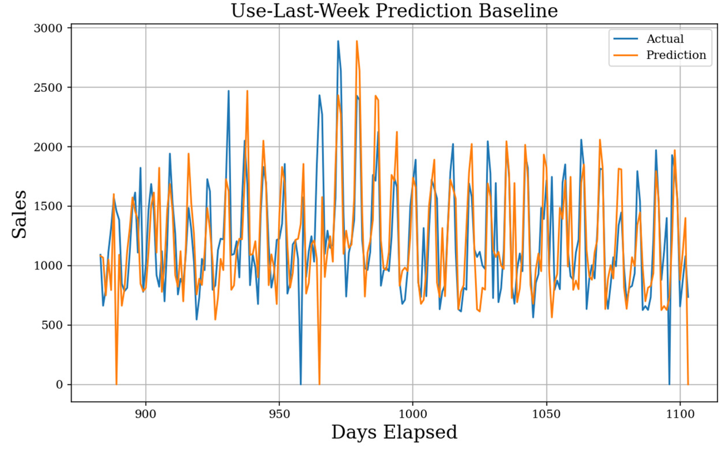
Figure 2. Use-Last-Week Prediction. Using the weekly seasonality, the next prediction baseline expects day D (t) is exactly the previous weekday D (t − 7). The MAE baseline generated is 278, and the prediction shape fails when experiencing extreme values.

In Figure 3, it was seen that the result of the Use-Last-Week-Enhanced prediction. The MAE score for the prediction is 239 showing a large improvement over simpler baselines and is even sensitive to change over time as short-term increases or decreases will be caught by the next week. This simple model boasts a sMAPE of 21.5%, which is very good. Although it is sensitive to changing patterns, the prediction will never propagate error from a holiday forward as badly as the other baselines.

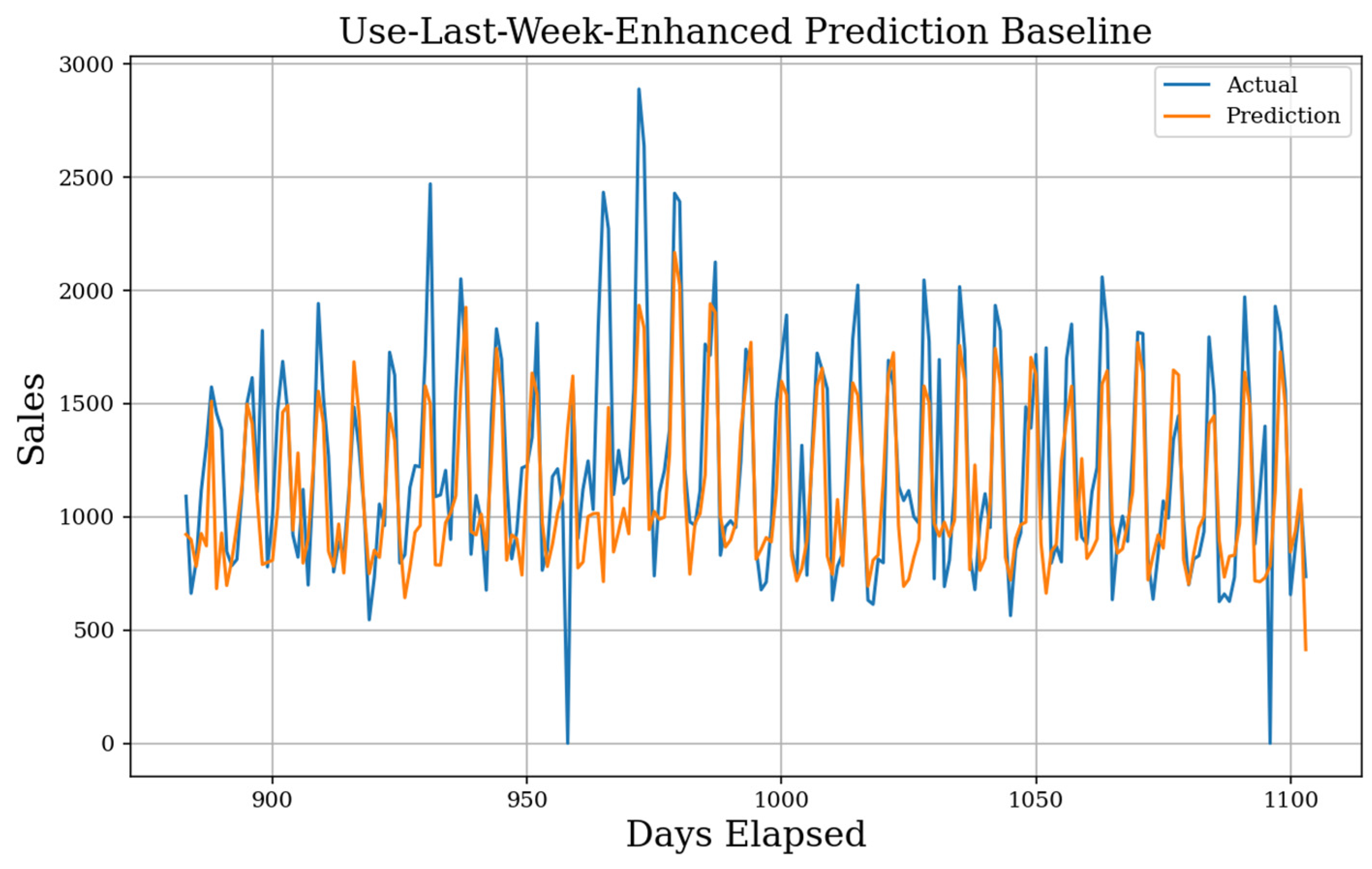
Figure 3. Enhanced Use-Last-Week Actual Prediction. Using the weekly seasonality and the mean weekday average, the final prediction baseline implements a simple history. The MAE baseline generated is 239, the sMAPE is 21.5%, and the gMAE is 150.

3. Feature Test Results

Figure 4 shows the rankings of the top 25 features in the actual dataset and their associated F-Scores. This ranking step is completed for each of the actual, daily differenced, and weekly differenced datasets and the results can be seen in the Supplementary Materials Figures S10–S12. Since the Temporal Fusion Transformer (TFT) model injects static context and does not need the 14 days of previous sales, we also give the top feature rankings with the 14 days removed in Supplementary Materials Figures S13–S16. Examining the results of the actual dataset, we see by far the most highly correlated features are the weekly average sales, the sales from one week ago, and the sales from two weeks ago. One feature of note, the year scores high, even though predicting sales by the year is not a good metric in reality. Since the actual dataset has a built-in trend, the feature seems more contextual than it really is. The daily differenced dataset, which has successfully removed trend, shows the highest scoring features as Monday and Saturday, as well as sales from one and two weeks ago as before. Although scores are not at high as before, there is still a good correlation, and features relying on trends do not rank highly such as before. Finally, the weekly differenced rankings show further diminished F-Scores. Sales from the day one week prior remain a consistent, highly correlated feature. Since the most correlation between instances has been removed by weekly differencing, holidays are ranked more highly than most other features.

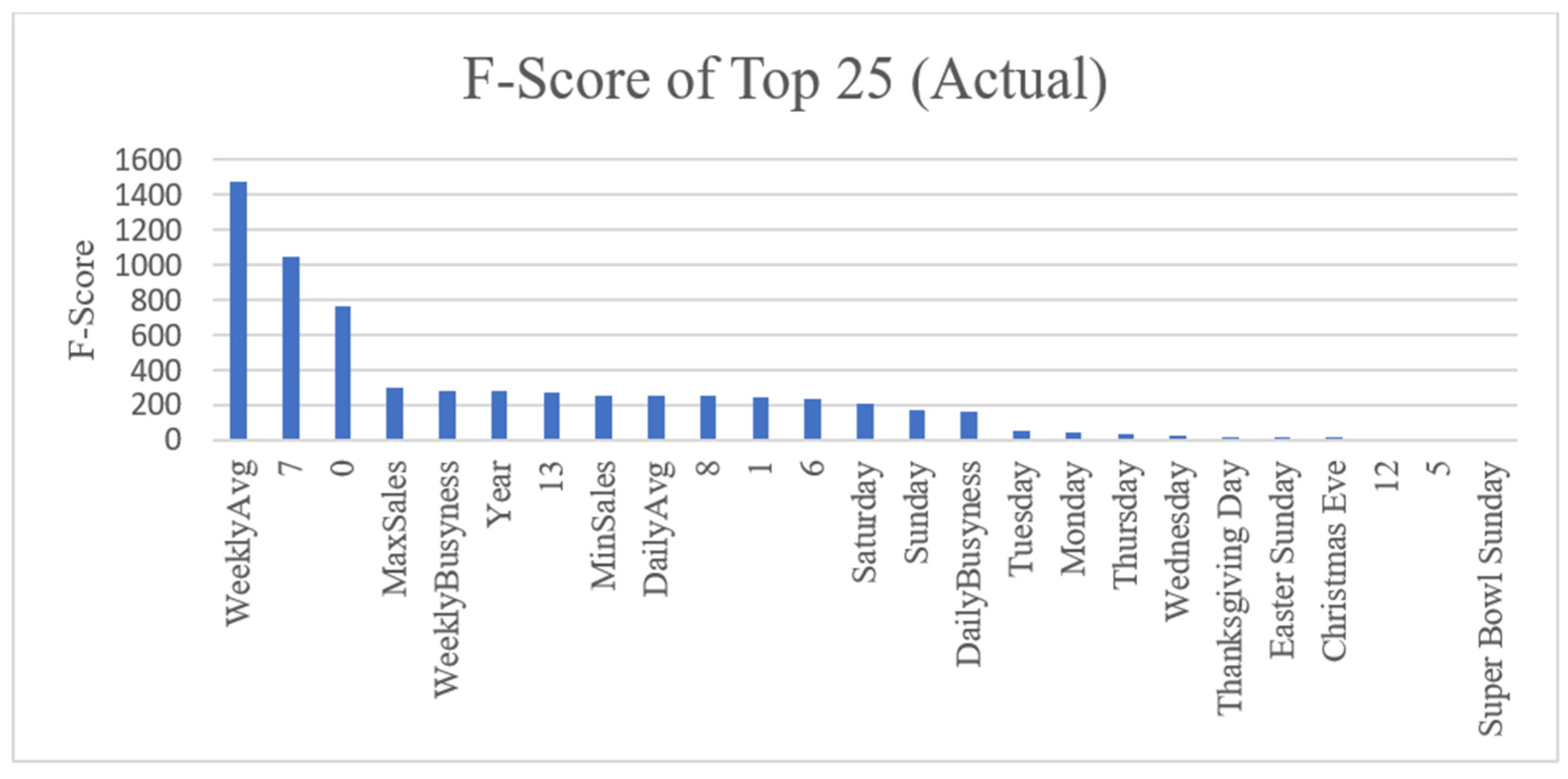
Figure 4. F-score for Top Features (Actual). The top 25 features as ranked by their F-scores. Weekly sales average is the highest scoring feature by far with other statistical metrics and days of the week following. Numbers 0–13 mark how many days until removal from the prediction window, so temporarily 13 is yesterday, 7 is one week ago, and 0 is two weeks ago.

The test to find the optimal number of features is completed for each model on each of the actual, daily differenced, and weekly differenced datasets for one-day and one-week forecast horizons. First, the one-day results was examine, followed by the extension to one-week. Figures for one-day results beyond the actual dataset can be seen in Supplementary Materials Figures S16–S21. The one-day actual feature test, shown in Figure 5, shows very promising results for the RNN models with LSTM using 22 features and GRU using 10, both scoring higher than other models. Other than some ensemble and linear non-RNN methods, most models received the highest MAE score from a smaller number of features on the actual dataset due to the high correlation of just a few features. This behavior is seen clearly in Figure 6 where all RNN models perform much worse after selecting more than 20 features. The one-day daily differenced feature test shows worse MAE scores overall, and the RNN models perform severely worse. Due to daily differencing linearly separating each instance, the best performing models may make use of more features. Kernel Ridge regression with 72 features received the best MAE in this stage and is comparable to the best results in the actual dataset. Ridge regression steadily decreased in MAE as the features increased, but RNN models fluctuated with an upward trend instead of improving, giving the best results with fewer features. The final weekly differenced one-day feature test gives steadily worse results for all models, and the RNN models are outperformed again by most other ML methods. For most models, except for some tree-based methods, the MAE never decreases beyond adding a small sampling of features, around 14 features for many models. For one-day feature testing, the best results was acquired overall from the actual data using few features and daily differenced data using many features, with the weekly differenced results underperforming overall with a middling number of features.

Figure 5. Best One-Day Forecast MAE Found Across 73 Features (Actual). Recurrent (orange) and non-recurrent (blue) models are trained with an iteratively increasing number of ranked features, seen in Supplementary Materials Figure S10, for one-day forecasting. The lowest MAE for each model is recorded with the number of features next to the model’s name.

Figure 6. All RNN Models and Ridge One-Day Forecast MAE Across 73 Features (Actual). We show how the number of features affects the MAE score for one-day forecasting in the actual dataset.

The one-week feature tests are comparable to the one-day tests in many cases, and the resulting figures can be examined in detail in the Supplementary Materials Figures S22–S27. Due to forecasting for seven time steps instead of just one, slightly higher MAE results overall was acquire . For the actual dataset, the LSTM model is still the best, with only 24 features included, and both GRU models performed very well. All high-scoring, non-recurrent models find the best results with an increased number of features, 60 or more in most cases. Although a high correlation was observed in features, most of the correlation is only useful for the t + 1th position, and the models need additional features to help forecast the remaining six days. Other than higher overall MAE scores and more features used on average, the results from the one-week feature test are very similar to the one-day results.

4. One-Day Forecasting Results

The best model for forecasting one-day into the future implements the kernel ridge algorithm with a test MAE of 214, sMAPE of 19.6%, and a gMAE of 126, although all 25 top models are shown in Table 1. The dataset used was the daily differenced dataset, and the forecast result is seen in Figure 7. This is the best individual MAE score among all models. The TFT model with fewer features forecasted over the actual dataset also did well with an MAE of 220, sMAPE of 19.6%, and a gMAE of 133. This model better captures special day behaviors but is less adaptive since it uses fewer features. The ensemble Stacking method also received good results using the actual dataset, making it comparable to the TFT model. Otherwise, many models outperformed the best Use-Last-Week-Enhanced baseline. When examining datasets, daily differencing consistently achieves scores higher than the actual or weekly differenced dataset, especially with linear models. RNN models require the actual dataset to achieve results which are better than the baseline and still perform worse in some cases. The actual dataset still achieves below baseline results with other ML models as well; they are just not as good as seen when differencing daily. Finally, the weekly differenced dataset provides results almost entirely worse than the baseline, with the best result coming from the Voting ensemble. The full table of test results with all models is given in Supplementary Materials Table S9, and there are figure examples from high performing or interesting forecasts in Supplementary Materials Figures S28–S35.

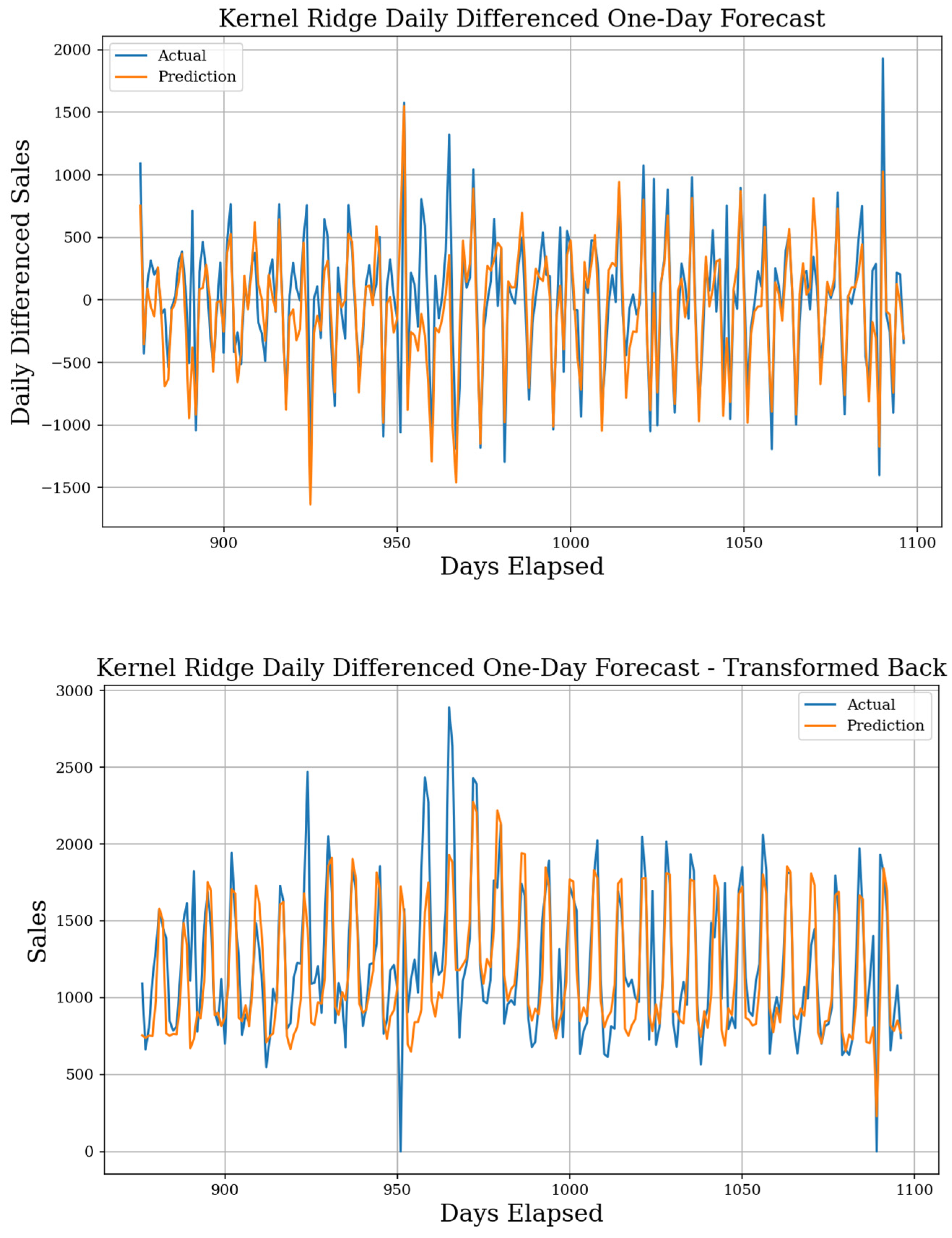
Figure 7. Kernel Ridge Daily Differenced One-Day Forecast. MAE of 214, sMAPE of 19.6%, and gMAE of 126, with 72 features. Original predictions (top) and the transformed back version (bottom) are both shown. This shows the best performing one-day forecast.

Table 1. Top 25 One-Day Forecast Results. It shows the top 25 results for one-day forecasting from all tests, sorted by dataset, then ranked from best to worst. The model, test MAE, sMAPE, gMAPE, and the dataset used to achieve the result are all given. Some best and worst results from each dataset and the baseline are highlighted. The table is sorted by MAE then dataset, and the best results are seen in the Actual and Daily datasets.

Model	Type	MAE	sMAPE	gMAE	Dataset
Stacking	NR	220	0.195	142	Actual
TFT Less Features	R	220	0.196	133	Actual
Bayesian Ridge	NR	221	0.195	144	Actual
Linear	NR	221	0.195	144	Actual
Ridge	NR	221	0.195	144	Actual
SGD	NR	221	0.195	144	Actual
LSTM	R	222	0.196	131	Actual
Lasso	NR	226	0.201	147	Actual
GRU	R	227	0.2	144	Actual
Extra Trees	NR	231	0.204	128	Actual
Use-Last-Week-Enhanced	NR	239	0.215	150	Actual
TFT All Features	R	244	0.215	159	Actual
Kernel Ridge	NR	214	0.196	126	Daily
Ridge	NR	216	0.195	144	Daily
Bayesian Ridge	NR	217	0.196	146	Daily
Linear	NR	219	0.198	137	Daily
Lasso	NR	223	0.201	141	Daily
Stacking	NR	223	0.2	148	Daily
XGB	NR	241	0.214	152	Daily
Voting	NR	238	0.213	144	Weekly
Stacking	NR	242	0.215	139	Weekly
Bayesian Ridge	NR	245	0.218	142	Weekly
Kernel Ridge	NR	245	0.219	144	Weekly
Linear Regression	NR	245	0.217	140	Weekly
Lasso	NR	246	0.218	141	Weekly

5. One-Week Forecasting Results

When reviewing Table 2, the best model MAE score over one-week is the TFT model with fewer features achieving an MAE of 219, sMAPE of 20.2%, and a gMAE of 123 using the actual sales dataset. The forecast, seen in Figure 8, shows a perfect capture of the two holidays. However, the GRU and LSTM models both achieve a better sMAPE of 19.5% and 19.7%, respectively, and they both have better gMAE scores. The GRU model is hindered by a very high deviation between the starting days, and a Sunday start gave the best results. No other results achieved better scores than the Use-Last-Week-Enhanced baseline. The best performing non-recurrent models were ensemble methods Extra Trees, Stacking, and Voting, all on the actual dataset. When examining datasets, the only results better than the baselines came from the Actual dataset. Although, it is likely most accurate to say that only the recurrent algorithms performed well, and the actual dataset is the only one conducive for training recurrent models. The weekly differenced dataset does perform better than the daily differenced dataset here in terms of MAE, although the sMAPE is massive. Examining the forecasts shows models which are predicting close to zero-difference to achieve results approaching the Use-Last-Week baseline, which explains decent MAE but high sMAPE. The daily differenced dataset is not capable of making good predictions when using this forecasting method on a long window. The best result is the Lasso model with only an MAE of 280, sMAPE of 101.6%, and a gMAE of 162. The full table of test results with all models is given in Supplementary Materials Table S10, and there are some figure examples from high performing or interesting forecasts in Supplementary Materials Figures S36–S43.

Figure 8. Transformer Less Features Actual One-Week Forecast. The best start day MAE of 216 is found when starting on Tuesday. A sMAPE of 20.2% and gMAE of 123 show it may look for more improvements in the future, as results are not as good overall as one-day. A mean MAE of 218 and a standard deviation of 1.29 are found with 17 features. TFT perfectly captures the two holiday zero-sale days without acknowledging the zero-sale ‘hurricane day’.

Table 2. Top 25 One-Week Forecast Results. It shows the top 25 results for one-week forecasting from all tests, sorted by dataset, then ranked from best to worst. The model, test MAE, sMAPE, gMAPE, and the dataset used to achieve the result are given. One-week specific metrics such as best start day, the mean of each weekday start, and the standard deviation between each start are also included. Best results are bolded. RNN models with the Actual dataset are the only results to beat the baseline Use-Last-Week-Enhanced. Alternate methodologies for extending non-RNN models to longer horizon windows must be explored further and sorted by MAE then dataset.

Model	Type	MAE	sMAPE	gMAE	Dataset	Weekday	Mean	Std Dev
TFT Less Features	R	215	0.202	123	Actual	Friday	222	3.363
GRU	R	218	0.195	116	Actual	Sunday	233	13.477
LSTM	R	222	0.197	134	Actual	Thursday	228	5.339
Use-Last-Week-Enhanced	NR	230	0.203	139	Actual	Tuesday	232	2.437
GRU+	R	233	0.204	136	Actual	Wednesday	246	14.612
ExtraTrees	NR	235	0.206	145	Actual	Wednesday	240	4.085
Stacking	NR	237	0.208	146	Actual	Tuesday	243	4.634
Voting	NR	237	0.209	140	Actual	Friday	246	8.256
Kernel Ridge	NR	239	0.213	143	Actual	Wednesday	244	4.229
SGD	NR	240	0.214	140	Actual	Tuesday	249	7.712
Bayesian Ridge	NR	242	0.216	145	Actual	Wednesday	248	3.408
Lasso	NR	243	0.218	147	Actual	Thursday	248	2.979
Transformer	R	267	0.239	153	Actual	Wednesday	268	1.131
Lasso	NR	280	1.016	162	Daily	Sunday	287	6.53
Lasso	NR	253	1.284	137	Weekly	Sunday	256	3.156
Ridge	NR	256	1.274	144	Weekly	Sunday	261	3.403
Kernel Ridge	NR	257	1.274	146	Weekly	Sunday	262	3.436
Elastic	NR	257	1.327	153	Weekly	Sunday	259	1.495
SGD	NR	257	1.28	148	Weekly	Monday	261	2.978
LinSVR	NR	258	1.405	149	Weekly	Sunday	260	1.939
Bayesian Ridge	NR	259	1.304	151	Weekly	Sunday	260	1.21
Stacking	NR	260	1.281	151	Weekly	Monday	264	2.694
Transformer	R	263	1.371	147	Weekly	Tuesday	278	9.849
RNN	R	273	1.722	162	Weekly	Sunday	278	2.95
GRU	R	273	1.674	154	Weekly	Sunday	279	4.318

Supplementary Materials

Supplementary materials are available online at https://www.mdpi.com/article/10.3390/make4010006/s1,

References

Green, Y.N.J. An Exploratory Investigation of the Sales Forecasting Process in the Casual Themeand Family Dining Segments of Commercial Restaurant Corporations; Virginia Polytechnic Institute and State University: Blacksburg, VA, USA, 2001.
Cranage, D.A.; Andrew, W.P. A comparison of time series and econometric models for forecasting restaurant sales. Int. J. Hosp. Manag. 1992, 11, 129–142.
Lasek, A.; Cercone, N.; Saunders, J. Restaurant Sales and Customer Demand Forecasting: Literature Survey and Categorization of Methods, in Smart City 360°; Springer International Publishing: Cham, Switzerland, 2016; pp. 479–491.
Green, Y.N.J.; Weaver, P.A. Approaches, techniques, and information technology systems in the restaurants and foodservice industry: A qualitative study in sales forecasting. Int. J. Hosp. Tour. Adm. 2008, 9, 164–191.
Lim, B.; Arik, S.O.; Loeff, N.; Pfister, T. Temporal Fusion Transformers for Interpretable Multi-horizon Time Series Forecasting. arXiv 2019, arXiv:1912.09363.
Borovykh, A.; Bohte, S.; Oosterlee, C.W. Conditional Time Series Forecasting with Convolutional Neural Networks. arXiv 2018, arXiv:1703.04691.
Lim, B.; Zohren, S. Time-series forecasting with deep learning: A survey. Philos. Trans. R. Soc. 2021, 379, 20200209.
Bandara, K.; Shi, P.; Bergmeir, C.; Hewamalage, H.; Tran, Q.; Seaman, B. Sales Demand Forecast in E-commerce Using a Long Short-Term Memory Neural Network Methodology. In International Conference on Neural Information Processing; Springer: Berlin/Heidelberg, Germany, 2019; pp. 462–474.
Helmini, S.; Jihan, N.; Jayasinghe, M.; Perera, S. Sales forecasting using multivariate long short term memorynetwork models. PeerJ PrePrints 2019, 7, e27712v1.
Makridakis, S.; Spiliotis, E.; Assimakopoulos, V. Statistical and Machine Learning forecasting methods: Concerns and ways forward. PLoS ONE 2018, 13, 3.
Stergiou, K.; Karakasidis, T.E. Application of deep learning and chaos theory for load forecastingin Greece. Neural Comput. Appl. 2021, 33, 16713–16731.

© Text is available under the terms and conditions of the Creative Commons Attribution (CC BY) license; additional terms may apply. By using this site, you agree to the Terms and Conditions and Privacy Policy.

Upload a video for this entry

Information

Subjects: Computer Science, Artificial Intelligence

Contributor MDPI registered users' name will be linked to their SciProfiles pages. To register with us, please refer to https://encyclopedia.pub/register :

Md Tamjidul Hoque

View Times: 1.4K

Update Date: 10 Feb 2022

Table of Contents

Video Upload Options

Confirm