Your browser does not fully support modern features. Please upgrade for a smoother experience.
Submitted Successfully!
 +1 credit
Thank you for your contribution! You can also upload a video entry or images related to this topic.
For video creation, please contact our Academic Video Service.
| Version | Summary | Created by | Modification | Content Size | Created at | Operation |
|---|---|---|---|---|---|---|
| 1 | Katarzyna Kopczewska | + 3567 word(s) | 3567 | 2022-01-16 09:16:03 | | | |
| 2 | Jessie Wu | Meta information modification | 3567 | 2022-01-18 02:27:50 | | |
Video Upload Options
We provide professional Academic Video Service to translate complex research into visually appealing presentations. Would you like to try it?
Cite
If you have any further questions, please contact Encyclopedia Editorial Office.
Kopczewska, K. Prediction of Customer Churn in Retail E-Commerce Business. Encyclopedia. Available online: https://encyclopedia.pub/entry/18374 (accessed on 23 July 2026).
Kopczewska K. Prediction of Customer Churn in Retail E-Commerce Business. Encyclopedia. Available at: https://encyclopedia.pub/entry/18374. Accessed July 23, 2026.
Kopczewska, Katarzyna. "Prediction of Customer Churn in Retail E-Commerce Business" Encyclopedia, https://encyclopedia.pub/entry/18374 (accessed July 23, 2026).
Kopczewska, K. (2022, January 17). Prediction of Customer Churn in Retail E-Commerce Business. In Encyclopedia. https://encyclopedia.pub/entry/18374
Kopczewska, Katarzyna. "Prediction of Customer Churn in Retail E-Commerce Business." Encyclopedia. Web. 17 January, 2022.
Copy Citation
Customer Relationship Management (CRM) is defined as a process in which the business manages its interactions with customers using data integration from various sources and data analysis.
churn analysis
customer relationship management
machine learning
1. Background
Maintaining high customer loyalty is a common challenge in business. Multiple studies [1][2][3] have proved that retaining customers is more profitable than acquiring new ones. Customer Relationship Management (CRM) deals with loyalty, or oppositely, churn prediction. Most of the previous studies have been conducted for industries in which customers are tied with contracts (such as telecom [4] or banking), which limits the churn rate. Many studies show that customer churn can successfully be predicted using a Machine Learning approach [5][6][7].
2. Customer Churn in CRM and Modelling
Improving the loyalty of the customer base is profitable to the company. This has its source in multiple factors, where the most important one is the cost of acquisition. Numerous studies have proved that retaining customers costs less than attracting new ones [1][2][3]. Moreover, there is some evidence that loyal customers are less sensitive to competitor actions regarding price changes [8][9].
There are two basic approaches for companies dealing with customer churn. The first one is an “untargeted” approach. This is where a company seeks to improve its product quality and relies on mass advertising to reduce the churn. The other method is a “targeted” approach, where the company tries to aim their marketing campaigns at the customers who are more likely to churn [10]. This approach can be divided further by how the targeted customers are chosen, for example, the company can target only those who have already decided to resign from another relationship. In contractual settings, this can mean cancelling a subscription or breaching a contract. Another way to approach the churn problem is to predict which customers are likely to churn soon. This has the advantage of having lower costs, as the customers who are about to leave are likely to have higher demands from any last-minute deal proposed to them [11].
A literature review demonstrates [11] that most studies concerning churn prediction have been performed in contractual settings, where churn is defined as the client resigning from using a company’s services by cancelling their subscription or breaching the contract. This way of specifying churn is different from a business setting, where the customer does not have to inform the company about resigning.
One problem that arises in the non-contractual setting is the definition of churn. As there is no precise moment when the customer decides not to use the company’s services anymore, it must be specified by the researcher based on the goals of the churn analysis. One can label customers as “partial churners” when they do not make any new purchases from the retail shop for three months [12]. In other approaches, “churners” are all the customers who have a below-average frequency of purchases [3] since these customers have been shown to provide little value to the company. In the case of this study, customers were classed as churners if they never bought from the shop again after their first purchase.
3. Results of the Pre-Modelling Phase
Topic modelling was used to extract meaningful information from the customer’s text reviews. The resulting topic assignments should help us to validate if customer perception is important for their propensity to churn. Moreover, such data can be used in other parts of CRM, such as live monitoring of customer satisfaction. The topics obtained from LDA, Gibbs Sampling and aspect extraction methods were manually assessed. In LDA and Gibbs Sampling, the topic assignments were not coherent, and the models were not able to infer topics meaningfully. The only reasonable output was produced by the last method, attention-based aspect extraction. For some of the inferred topics, all the reviews had similar content—for example, one topic included reviews which praised fast delivery (“On-time delivery”), and another contained short positive messages about the purchase (“OK”). An interesting remark is that “spam” reviews (e.g., “vbvbsgfbsbfs”, “Ksksksk”) were also classified into one topic. This suggests that topics are correctly inferred by the aspect extraction method, and the variables indicating topic assignments can improve the machine learning model. The topic modelling results with examples of reviews for each topic. Technically, attention-based aspect extraction was superior to latent Dirichlet allocation and its improved version and can probably discover topics better in the case of short texts. Nevertheless, using LDA is considerably easier, as this method is widely popular with a good coverage of documentation and easy-to-apply implementations. On the other hand, aspect extraction requires some level of expertise regarding neural network modelling. The available implementation requires some changes to the code so that it works on a dataset other than the one used in the original study. Besides that, neural network model training takes a couple of hours, while for LDA it takes only twenty minutes.
Customer density, obtained with the DBSCAN algorithm, divided customers into groups living in rural (sparsely populated) or urban (densely populated) areas. This information was then included in the machine learning model to test if customers from rural areas are less prone to churn. Visual inspection the assignment of customers to DBSCAN density clusters showed that the boundaries of the clusters overlapped with the boundaries of bigger cities, which proves that the clustering inferred densely populated areas correctly.
PCA-dimension reduction was applied to 36 geodemographic features to reduce the number of features that the models would have to learn, while retaining most of the information from the original set of features. The first 10 most informative PCA eigenvectors (loadings) accounted for 97.3% of the explained variance. Such a high value of explained variance means that applying the PCA transformation was successful in data compression and information preservation. Consequently, the first 10 eigenvectors (instead of 36 features) were included as explanatory variables in the modelling phase, which greatly reduced the model complexity and training time.
4. Performance Analysis
AUC metric analysis was used to compare all XGBoost and LR models tested in this study, which differed in terms of the sets of independent variables used (Table 1). All models used the same dependent variable, which was an indicator of whether the customer had placed a second order. The best AUC score in the test set was achieved by the XGBoost model with basic features combined with dummies which indicated the product categories that the customer bought during their first purchase. Its AUC was greater than 0.5, which means that the model has a predictive power better than random guessing. The second best XGB model contains all variables, with PCA-transformed demographic variables and product categories; thus, similar performance is not surprising. The percentage drop in AUC between the first and second XGB model is very small (0.6%). The model with only basic information is about 2.5% worse. The AUC score of the model based on Boruta-selected features is 0.646% less than the model, including all variables. This means that using the Boruta algorithm did not bring additional predictive power to the model. The model with review topics performed better than without them, making review topics relevant to model performance. In the case of the Logistic Regression (LR) models, the main finding is that even the best LR model (containing product categories and basic features) performed worse than the worst XGBoost model (0.586 vs. 0.625, respectively), and the ranking of models changed. This suggests that linear modelling is, in general, very poorly suited for this prediction task. AUC values for the LR model test set oscillate below 0.6, which means that the models are very poorly fitted to the data. The worst LR model (AUC test = 0.546), with the agglomeration (population) feature only, shows performance very close to the random classifier (AUC test = 0.5), so one could argue that this model does not have any predictive power. Interestingly, based on AUC values, both the LR and XGBoost models use the same features fir the highest-performing models—namely product categories and all variables. This suggests that these variables provide the biggest predictive power, regardless of the model used. The second interesting remark comes from comparing the models based on an agglomeration set of features (population density indicator). In the XGBoost model, this feature is rated as the third most informative (after excluding the Boruta set to compare meaningfully with the LR table), while it is scored as the least informative in the case of LR. One possible explanation is the inherent ability of XGBoost to create interactions between variables, while these interactions need to be included in LR models manually.
Table 1. AUC values for XGBoost and logistic regression models.
| AUC Test | AUC Train | Performance Drop vs. the Best Model | ||||
|---|---|---|---|---|---|---|
| Model with Included Basic Variables and… |
XGB | LR | XGB | LR | XGB | LR |
| Product categories | 0.6505 | 0.5862 | 0.9995 | 0.5922 | 0.00% | 0.00% |
| All remaining variables | 0.6460 | 0.5813 | 0.9997 | 0.5960 | −0.68% | −0.84% |
| Features selected by Boruta algorithm | 0.6426 | 0.5801 | 0.9998 | 0.5912 | −1.20% | −1.05% |
| Population density indicator | 0.6382 | 0.5464 | 0.9993 | 0.5532 | −1.88% | −6.79% |
| Review topics | 0.6353 | 0.5639 | 0.9992 | 0.5595 | −2.34% | −3.81% |
| Nothing more | 0.6338 | 0.5535 | 0.9991 | 0.5529 | −2.56% | −5.58% |
| Geodemographics (with PCA) | 0.6323 | 0.5482 | 0.9996 | 0.5606 | −2.80% | −6.48% |
| Geodemographics (without PCA) | 0.6254 | 0.5492 | 0.9995 | 0.5632 | −3.86% | −6.31% |
Note: The table was sorted by highest-performing XGB models. The final columns show the percentage change in performance compared to the best-performing model.
From a CRM perspective, the most important result of the modelling procedure is that the created models have predictive power for churn prediction. This means that by using the model’s predictions, a firm can forecast which customers are most likely to place a second order and can be encouraged further; and on the other hand, which customers have a very low probability of buying and whom the company should restrain from targeting to save money.
The AUC scores in Table 1 are the point estimates. One cannot guess if the performance would still be the same for a slightly different test set from such information. This is especially crucial in the case of this study, as the differences between all the XGBoost models are not large. A standard way to compare the models’ performance more robustly is using a bootstrapping technique. Observations from the test set were sampled with replacement (100 re-sample rounds), and the AUC measure was calculated with the density function. This again provided a ranking of the models (Figure 1) demonstrating that the best model used product categories and basic information, the second best used all variables, and the baseline used only basic information. The curve for the model with basic features stands out from the others. However, the difference between the highest- and second highest-performing models is not as clear—it looks like the better model has a slightly better density curve shape, but this should be investigated more thoroughly. With the Kolmogorov-Smirnov (K-S) test, whether the empirical distributions came from the same probability distribution. This is a non-parametric test to assess whether two empirical samples come from the same distribution. The K-S statistic is calculated based on the largest distance between the empirical distribution functions of both samples, and this statistic is then compared against the Kolmogorov distribution. The null hypothesis in this test is that two samples come from the same underlying distribution. The test was run twice using two alternative hypotheses. The first one with H1: auc_best =/= auc_2nd_best, and the second one: H1: auc_best > auc_2nd_best. The p-value for the first hypothesis was 0.0014, which suggests that models are distinguishable. The p-value for the second hypothesis was 0.0007, which confirms that the performance of the first model (only product categories) is significantly better than that of the second one (all variables).
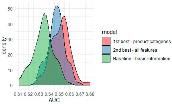
Figure 1. Bootstrap AUC estimates for three XGBoost models.
Aside from the statistical justification for choosing the smaller model (with fewer variables), the theory of Occam’s razor heuristic is relevant. The model with product categories has 21 variables, while the one with all variables includes 47. If there is no important reason for why the more complex approach should be used, the simpler method is usually preferable. In this case, using a simpler model has the following advantages for usage in a CRM context. First, it provides faster inference about new customers—especially in an online prediction setting when predictions must be made on the fly. Secondly, the projections are easier to interpret, and thirdly, it is easier to train and re-train the model.
Lift metric analysis computes the likelihood of re-purchase in ranked groups of customers. More specifically, one creates a ranking of customers in which they are sorted by their likelihood to buy for a second time. For each cumulative group in the ranking (the top 1% of customers, the top 10%, etc.), one can compute which percentage of this group is truly buying for the second time. An ultimate goal of customer churn prediction is gaining information on which customers are most likely to place a second order. Lift metric analysis is a go-to tool for measuring the performance of targeting campaigns. It is also very easily understood by CRM experts without a deep knowledge of statistics and machine learning.
Technically, in lift metric analysis, customers are divided into segments defined as the top x% of the ranking which is output by the targeting model. The procedure for calculating the lift metric, for example, of the top 5% of customers, is defined as follows:
-
Sample 5% of all customers. Calculate the share of these customers (share_random), who have a positive response (who truly bought for a second time).
-
Using a machine learning model, predict the probability of buying for a second time all the customers. Then, rank these customers by the likelihood and select the top 5% with the highest probability. Calculate the share of these customers (share_model) who have a positive response.
-
Calculate the lift measure as share_model/share_random. If the lift value is equal to one, this means that the machine learning model is no better at predicting the top 5% of the best customers than random guessing. The bigger the value, the better the model is in the case of this top 5% segment. For example, if the lift metric is equal to three, the model is three times better at targeting promising customers than random targeting.
Such calculations can be repeated for multiple customer segments, typically defined by the top x% of the ranking. CRM experts can then consider lift values for various segments, combine this insight with targeting cost, and decide what percentage of the customers should be targeted.
A lift curve (Figure 2) is convenient for visualising lift metrics for multiple segments at once, with a fraction of top customers ranked by probability to re-purchase on the x-axis and lift value on the y-axis. The shape of the plot resembles the 1/x function. The lift values are very big for the smallest percentage of the best customers to target, and they get smaller quickly. This means that the more customers the company would like to target based on the model’s prediction, the less marginal the effects would be from using the model. For example, for the top 1% of customers, the model can predict retention 18.7 times better than a random targeting approach. It is still very effective for the top 5%, being 4.2 times better than random. If one wants to target half of the customers, the improvement over random targeting is 0.3 (130%), and although this value is less impressive than for smaller percentages, it is still an improvement over random targeting.
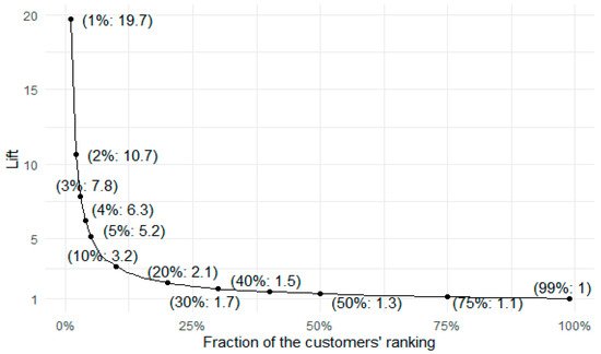
Figure 2. Lift curve for best XGBoost model.
5. Understanding Feature Impact with Explainable Artificial Intelligence
Discovering which features to use and how to drive the predictions of customer churn/loyalty is very important for successful CRM. Permutation-based variable importance is first employed to check if particular sets of features have any influence on the model’s predictions, and if they do, how strong this influence is. Secondly, the partial dependence profile technique is used to check the direction of this influence.
Permutation-based Variable Importance (VI) was assessed for the two best XGBoost models (with all variables and with basic features and product categories). VI can answer questions about the impact of particular sets of variables. The variables were grouped into five sets:
-
behavioural—variables describing the first transaction of the customer: payment value, product category, etc.
-
perception—variables describing quantitative revives (on a scale of 1–5) and dummies for textual (topic) reviews.
-
“geo” variables—with three subgroups:
- ○
-
demographic variables describing the population structure of a customer’s region.
- ○
-
raw location, being simply longitude/latitude coordinates.
- ○
-
density variable, indicating whether the customer lives in a densely populated area.
Considering all variables in the five thematic groups (Figure 3), the best set of variables contains the behavioural features. The following two sets, geo-demographic and raw spatial location, have a similar moderate influence. The perception variables (reviews) and the density population (rural/urban) indicator have the lowest impact on the model’s predictions. These results follow our expectations. A customers’ propensity to churn depends on: (i) payment value for the first order, number of items bought, shipping cost, (ii) categories of the products bought, (iii) demographic environment of the customer and (iv) customer location. At the same time, the customers’ propensity to churn is not influenced by: (i) population density in the customer’s area and division into rural and urban areas, (ii) quantitative review of the first purchase or (iii) qualitative review summarised as a topic.
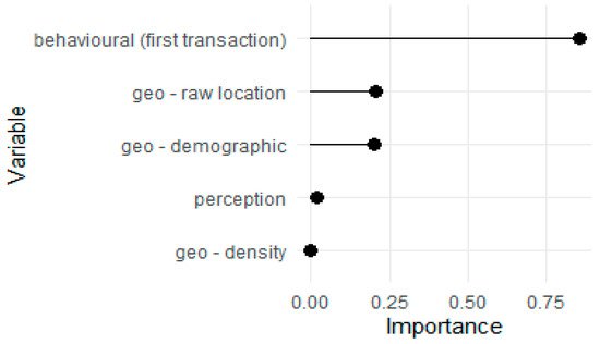
Figure 3. Variable importance plots for the model with all variables.
The second best XGB model which includes all variables reveals the detailed impact 1080 of all considered factors, individually (Figure 4a) and in groups (Figure 4b). The most important variables are the transportation cost, the value paid, and the geo-location provided by longitude and latitude. Most of the dummies which indicate product categories are in the latter part of the ranking. One can question why these features are ranked as relatively unimportant variables when they lead to a 2.5% gain in AUC compared to the model which does not used these features. This is because conceptually, all dummies which indicate product category are considered separately. The same effect is seen with geographic coordinates. To account for this, feature importance for these variable sets (“geolocation” and “prod_categories”) was used instead of individual feature importance. This information is presented in the right subfigure. After this operation, product categories gained relative importance to become the fourth most important variable, and the geolocation variable set becomes more important than payment value and transportation cost.
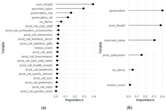
Figure 4. Variable importance plots for the model with all variables: (a) individual variables, (b) groups of variables.
Partial Dependence Profile (PDP) (Figure 5) allows for testing the direction and strength of the influence of various factors on customer churn. It was applied to payment value for the first order, the number of items purchased, customer location and review score. The PDP for payment value (Figure 5a) is non-monotonous. From an analysis of the smoothed model response (blue line), one can say that it continuous to increase until the point of around 100. This means that on average, until the payment value reaches 100, the bigger the payment value, the bigger probability of placing a second order by the customer as predicted by the model. After this threshold of 100, the probability of buying for the second time falls slowly. The PDP for the number of items purchased (Figure 5b) shows that the relationship between the number of items bought in the first purchase and the probability of the second purchase is negative—the more items purchased, the less likely the second purchase. One must remember that there is only one product in 80% of the orders, while in 10% there are two items. At the same time, the drop in the model’s response between one and two items is not very abrupt, meaning that this feature on its own cannot serve as a very good discriminator of customer churn for most of the observations. For CRM, information about such a relationship can lead to the following trade-off. The more the customer buys in the first purchase, the bigger the chance that they will not make a second purchase. This can have implications in cross-selling campaigns. The company can maximise the revenue from the first transaction by making the customer buy more, but then there is a bigger possibility that the customer will not make the second purchase. In the case of the PDP for geolocation data (Figure 5c), the predictions are the highest in two distinct areas—one having its centre close to Brasilia (the new capital of the country) and the other one on the same latitude but closer to the western country border. The predictions form a visible pattern in stripes, which comes from a limitation of the model underlying the XGBoost method: decision trees [13]. A simple decision tree algorithm works by partitioning the feature space on a discrete basis. A typical output of such a model in 2D space is the formation of visible rectangles. Because XGBoost consists of stacked decision trees, the resulting partition pattern is a bit more complex, but decision-tree-typical artefacts are still visible. The PDP for review scores (Figure 5d) should be treated with caution, as variable importance assessment showed it to be relatively non-important, and the model response is relatively flat in reaction to changes in review score. For reviews which score one and two, the response does not change at all, meaning that it does not matter “how bad” the review is. Rather, it shows that unsatisfied customers will not buy again in general. With scores which range from two to five, the model response increases monotonically as is expected.
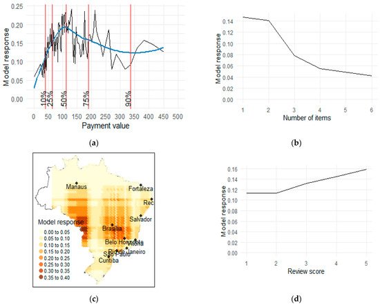
Figure 5. Partial dependence profiles for selected factors: (a) payment value of the purchase; (b) number of items in the customer’s purchase; (c) customer’s location; (d) 1–5 review score. Note: In panel (a) the blue line is a smoothed PDP curve.
References
- Dick, A.S.; Basu, K. Customer Loyalty: Toward an Integrated Conceptual Framework. J. Acad. Mark. Sci. 1994, 22, 99–113.
- Gefen, D. Customer Loyalty in e-Commerce. J. Assoc. Inf. Syst. 2002, 3, 2.
- Buckinx, W.; Poel, D.V.D. Customer base analysis: Partial defection of behaviourally loyal clients in a non-contractual FMCG retail setting. Eur. J. Oper. Res. 2005, 164, 252–268.
- Bach, M.P.; Pivar, J.; Jaković, B. Churn Management in Telecommunications: Hybrid Approach Using Cluster Analysis and Decision Trees. J. Risk Financ. Manag. 2021, 14, 544.
- Nie, G.; Rowe, W.; Zhang, L.; Tian, Y.; Shi, Y. Credit Card Churn Forecasting by Logistic Regression and Decision Tree. Expert Syst. Appl. 2011, 38, 15273–15285.
- Dalvi, P.K.; Khandge, S.K.; Deomore, A.; Bankar, A.; Kanade, V.A. Analysis of customer churn prediction in telecom industry using decision trees and logistic regression. In Proceedings of the 2016 Symposium on Colossal Data Analysis and Networking (CDAN), Indore, India, 18–19 March 2016; pp. 1–4.
- Gregory, B. Predicting Customer Churn: Extreme Gradient Boosting with Temporal Data. arXiv 2018, arXiv:1802.03396.
- Achrol, R.S.; Kotler, P. Marketing in the Network Economy. J. Mark. 1999, 63, 146.
- Choi, D.H.; Chul, M.K.; Kim, S.I.; Kim, S.H. Customer Loyalty and Disloyalty in Internet Re-tail Stores: Its Antecedents and Its Effect on Customer Price Sensitivity. Int. J. Manag. 2006, 23, 925.
- Burez, J.; Poel, D.V.D. CRM at a pay-TV company: Using analytical models to reduce customer attrition by targeted marketing for subscription services. Expert Syst. Appl. 2007, 32, 277–288.
- Tamaddoni Jahromi, A.; Sepehri, M.M.; Teimourpour, B.; Choobdar, S. Modeling Customer Churn in a Non-Contractual Setting: The Case of Telecommunications Service Providers. J. Strateg. Mark. 2010, 18, 587–598.
- Oliveira, V.L.M. Analytical Customer Relationship Management in Retailing Supported by Data Mining Techniques. Ph.D. Thesis, Universidade do Porto, Porto, Portugal, 2012.
- Behrens, T.; Schmidt, K.; Rossel, R.A.V.; Gries, P.; Scholten, T.; Macmillan, R.A. Spatial modelling with Euclidean distance fields and machine learning. Eur. J. Soil Sci. 2018, 69, 757–770.
More
Information
Contributor
MDPI registered users' name will be linked to their SciProfiles pages. To register with us, please refer to https://encyclopedia.pub/register
:
View Times:
3.3K
Revisions:
2 times
(View History)
Update Date:
18 Jan 2022
Table of Contents


Notice
You are not a member of the advisory board for this topic. If you want to update advisory board member profile, please contact office@encyclopedia.pub.
OK
Confirm
Only members of the Encyclopedia advisory board for this topic are allowed to note entries. Would you like to become an advisory board member of the Encyclopedia?
Yes
No
${ textCharacter }/${ maxCharacter }
Submit
Cancel
Back
Comments
${ item }
|
${ item.createdUser.fullName }
${ item.createdAt }
${ item.vote }
${ item.reply }
Delete
${ reply.createdUser.fullName }
${ reply.createdAt }
${ reply.vote }
Delete
There is no reply to this comment~
${ item.replyTextCharacter }/${ item.replyMaxCharacter }
Submit
Cancel
More
No more~
There is no comment~
${ textCharacter }/${ maxCharacter }
Submit
Cancel
${ selectedItem.replyTextCharacter }/${ selectedItem.replyMaxCharacter }
Submit
Cancel
Confirm
Are you sure to Delete?
Yes
No