Bone Tissues

Version	Summary	Created by	Modification	Content Size	Created at	Operation
1		Che-Yu Lin	+ 3070 word(s)	3070	2021-08-13 06:03:49	\|
2	format change	Lily Guo	-5 word(s)	3065	2021-09-13 03:37:51	\| \|
3	format change	Lily Guo	-5 word(s)	3065	2021-09-13 03:39:44	\|

This entry is adapted from the peer-reviewed paper 10.3390/ma14154224

Osseous tissue is a kind of hard connective tissue, which is also composed of cells, fibers and matrix. The fibers are bone glue fibers (the same as collagen fibers), and the matrix contains a large amount of solid inorganic salts.

bone tissue engineering hydrogel

1. Composition and Structure of Bone Tissue

In this section, we briefly review the composition and structure of a bone tissue. The content in this section is mainly referred to Refs. ^[1]^[2]^[3].

The mechanical properties of bone tissue, the primary tissue that makes up bone, are primarily determined by the composition and structure of bone tissue. It is important to remind that whole bone is actually an organ consisting of several different connective tissues including bone tissue. Please note that, in the context below, the term “bone” means “bone tissue” but not “bone organ”.

Compositionally speaking, bone is a composite material made up of organic and inorganic components. Organic components make up around 40% of the bone’s dry weight, and the primary organic component of bone is collagen fiber (mainly type I collagen). Inorganic components (in the form of mineral salts) make up around 60% of the bone’s dry weight, and the primary inorganic component is hydroxyapatite (a calcium phosphate–based mineral). Like other connective tissues, bone contains an abundant extracellular matrix. The organic and inorganic components construct the extracellular matrix of bone in a way that the framework of the extracellular matrix is formed by collagen fibers (organic components) while hydroxyapatite materials (inorganic components) are deposited on the framework for crystallizing and hardening the framework. The extracellular matrix of bone also contains around 25% water and several types of cells including osteoprogenitor cells, osteocytes, osteoblasts and osteoclasts.

Structurally speaking, bone has many small spaces (pores). Based on the size and density of the small space, bone can be categorized as two types, namely, compact bone (also called cortical bone) and spongy bone (also called trabecular bone), as shown in Figure 1. The relative quantity of each type differs among bones, but on average, compact bone and spongy bone constitute around 80% and 20% of the skeleton, respectively. These two types of bone have identical composition, but are different in structure macroscopically and microscopically. Compact bone forms the outer shell (or called cortex, and that is the reason why compact bone is also called “cortical” bone) of whole bone. The spaces within compact bone are much smaller; therefore, compact bone is much denser with a porosity of 5–10% and apparent density of 1.5–1.8 g/cm³ (that is the reason why it is called “compact” bone). Spongy bone is located at the end or on the inside of whole bone, and is surrounded by the outer compact bone. Spongy bone is composed of thin columns called trabeculae (that is the reason why spongy bone is also called “trabecular” bone), and is loose and less dense with a porosity of 50–90% and apparent density of 0.5–1.0 g/cm³. The porosity is one of the factors that strongly affect the mechanical properties of bone. Therefore, compact and spongy bones have significantly different mechanical properties because of their significant difference in the porosity. Compact bone can withstand much higher stress (up to about 150 MPa) but lower strain (up to about 3%) before failure, while spongy bone can withstand lower stress (up to about 50 MPa) but much higher strain (up to about 50%) before failure ^[4]^[5]^[6]^[7]^[8].

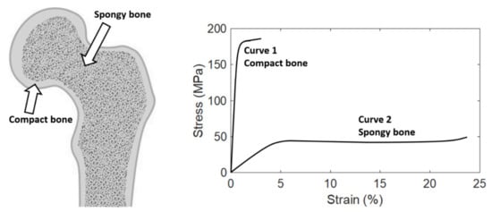
Figure 1. Left: Bone tissue can be categorized as two types, compact bone and spongy bone. Right: The typical stress–strain curves of compact and spongy bones. The last point of the stress–strain curve is the failure point. This figure is adapted from ^[3].

Normal whole bone is stiff and strong, but it is flexible and ductile, not brittle. This bidirectional mechanical behavior is contributed by the composition and structure of whole bone described above. Compositionally speaking, the inorganic components of bone make bone stiff and strong, while the organic components offer bone flexibility, ductility and toughness. Structurally speaking, compact bone is much stiffer and stronger than spongy bone, while spongy bone is more flexible and ductile. Therefore, the overall mechanical behavior of whole bone is the combination of these two diverse behaviors, making bone stiff and strong but at the same time flexible and ductile. This specialized mechanical behavior makes whole bone a versatile tissue having multiple mechanical functions, such as support, protection, and shock absorption.

2. Mechanical Properties of Compact Bone

In this section, we review the mechanical properties of compact bone that can be defined and extracted from the stress–strain curve measured using uniaxial tensile test until failure.

The stress–strain curve of a material represents the relationship between the stress and strain of that material under loading, and can be obtained by material testing system, either using uniaxial tensile or compression tests. The mechanical properties of a material can be obtained by analyzing the stress–strain curve of that material. For more information about the concepts of stress and strain as well as the standard method for obtaining the stress–strain curve of a material by a material testing system, please refer to ^[9].

The typical stress–strain curves of compact and spongy bones measured using uniaxial tensile test until failure are shown in Figure 1. It can be observed that the stress–strain curves of these two types of bone are quite different. Compact bone is much stiffer but more brittle than spongy bone. It means that compact bone can withstand much higher stress but less strain than spongy bone before failure. In addition, spongy bone can withstand much more energy (quantified by the area under the stress–strain curve) before failure, thanks to its porous structure.

The typical stress–strain curve of compact bone measured using uniaxial tensile test until failure is highlighted in Figure 2. It is important to note that this stress–strain curve is a bilinear, monotonically increasing curve. There are two linear curves in this bilinear curve, and that is the reason why a curve with this pattern is called a bilinear curve. The first linear curve (from points O to A, i.e., the linear curve within the elastic region) has a significantly greater slope than the second linear curve (from points B to C, i.e., the linear curve within the plastic region). Between the two linear curves is a short nonlinear curve. There are some regions and points associated with this stress–strain curve that have significant mechanical meanings, marked in Figure 2. These regions and points are closely related to the mechanical properties defined by the stress–strain curve. Below, we sequentially review a series of mechanical properties (listed in Table 1) of compact bone that can be defined and extracted from the stress–strain curve.

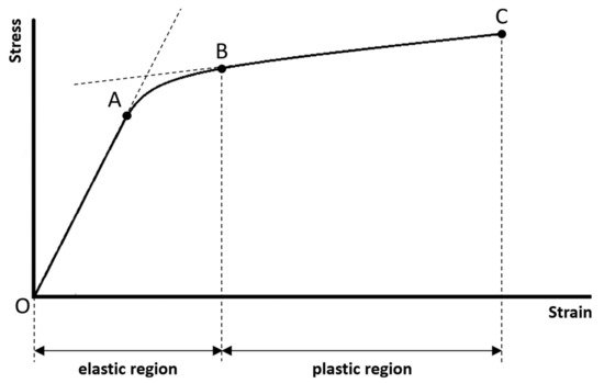
Figure 2. The typical stress–strain curve of compact bone measured using uniaxial tensile test until failure. Two regions (elastic and plastic regions) and four points (points O, A, B, and C) that have significant mechanical meanings are marked.

Table 1. Mechanical properties of compact bone that can be defined and extracted from the stress–strain curve.

(1) Range of the elastic region:

The elastic region is between points O (this is the origin of the stress–strain curve with zero stress and strain that indicates the instant of the beginning of loading) and B (the mechanical meaning of point B will be explained below). If the sample is loaded within the elastic region, the stress and strain will be completely recovered and back to zero once the applied loading is removed. There will be no permanent stress and strain, and the sample will be intact without any damages as well as compositional and structural changes, if the sample is loaded within the elastic region. In mechanics of material, the term “elasticity” is defined as the ability of a material to resume its original size and shape once the applied loading is removed. The greater the range of the elastic region, the greater the ability of the sample to reserve its elasticity.

(2) Range of the plastic region:

The plastic region is between points B and C (the mechanical meanings of points B and C will be explained below). If the sample is loaded beyond the elastic region and into the plastic region, there will be permanent strain (or called plastic strain) even though the applied loading is removed. The permanent strain is due to the permanent compositional and structural changes of the sample. It means that the sample will undergo damages as well as permanent compositional and structural changes, if the sample is loaded beyond the elastic region and into the plastic region. In mechanics of material, the term “plasticity” not only can imply damage and permanent strain, but also can imply ductility before failure. The greater the range of the plastic region, the greater the ductility of the sample. It means that the sample can undergo greater strain before failure; therefore, the sample may have a much lower chance to fail suddenly.

(3) Proportional limit:

The stress at point A is called the proportional limit. Although the proportional limit is not a point but actually means the stress at point A, one is accustomed to call it a point for the convenience of communication. Point A marks the end of the first linear curve. Between points O and A, the stress–strain curve is linear and is a straight line. It means that the stress and strain are linearly proportional on this curve. Beyond point A, the proportionality between the stress and strain no longer exists, and this is the reason why the stress at point A is called the proportional limit. In literature, some authors may assume that the proportional limit is equal to the elastic limit (the elastic limit will be explained below). It is reasonable to make such an assumption, since the proportional limit is often very close to the elastic limit for a material, although they are two different concepts. However, in this article, we suggest to assume that the proportional limit is not equal to the elastic limit.

(4) Elastic limit:

The stress at point B is called the elastic limit. Although the elastic limit is not a point but actually means the stress at point B, one is accustomed to call it a point for the convenience of communication. Point B marks the beginning of the second linear curve, also marks the end of the elastic region and the beginning of the plastic region. It means that point B is the boundary just between the elastic and plastic regions. This is the reason why the stress at point B is called the elastic limit. Beyond point B, the sample is loaded into the plastic region and undergoes damages as well as permanent compositional and structural changes. The stress and strain corresponding to point B are the largest stress and strain that can be applied to the sample without causing any permanent strain. If the sample is loaded beyond point B, it will not resume its original size and shape even though the applied loading is removed. It is important to note that most of the authors in literature prefer to use the term “yield point” to call point B, but not use the term “elastic limit”. However, we suggest that using the term “elastic limit” to indicate point B is more accurate, since point B marks the end of the elastic region. Besides, at least for compact bone, no significant yielding phenomenon (strain increases significantly while there is no observed increase in stress) can be observed on this stress–strain curve. It is also important to note that the elastic limit is seldom constantly defined in literature, and has been determined by different methods by different authors ^[10]. For example, the elastic limit is often defined as the same as proportional limit (point A). The offset method is another method sometimes used to determine the elastic limit, in which a line parallel to the first linear curve of the stress–strain curve is constructed, and the elastic limit is defined as the intersection of this line and the stress–strain curve. Please refer to ^[9] for more information about the offset method. In this article, we suggest to define the elastic limit as the beginning of the second linear curve (Point B).

(5) Failure strength:

Point C is called the failure point that marks the occurrence of the failure. The stress at point C is called the failure strength. In mechanics of materials, failure is defined as the state at which the sample completely breaks into more than one piece. The failure strength is the maximum stress that the sample can withstand before failure. The maximum stress in a stress–strain curve is called the ultimate strength; therefore, failure strength is equal to the ultimate strength in this case.

(6) Brittleness coefficient:

The brittleness coefficient is defined as the ratio of the strain at point B (i.e., the strain corresponding to the elastic limit) to the strain at point C (i.e., the strain where the failure occurs):

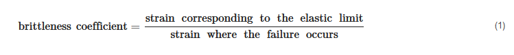
The brittleness coefficient is used to quantify how brittle the sample is, and it is a number between 0 and 1. The more the brittleness coefficient is close to 1, the more brittle the sample is. In order to understand what that means, it is important to remind what a brittle or a ductile material is. A material can be classified as either brittle or ductile in terms of how great the range of the plastic region is, compared to the range of the elastic region. A brittle material fails at a relatively low strain without undergoing a significant permanent strain, typically once the elastic limit is just reached. A ductile material undergoes a large permanent strain before failure. Therefore, the brittleness coefficient can be used to indicate the ratio between the range of the elastic region and the range of the plastic region. If the range of the elastic region is much greater than the range of the plastic region, the brittleness coefficient is greater, and the sample is more brittle.

(7) Modulus of resilience:

The modulus of resilience is the amount of energy per unit volume necessary to cause damages as well as permanent compositional and structural changes to the sample. The modulus of resilience is quantified by the area under the stress–strain curve in the elastic region (Figure 3). The greater the modulus of resilience, the greater the ability of the sample to absorb energy without permanent strain. The ability of a material to absorb energy without permanent strain is called resilience.

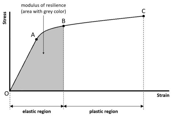
Figure 3. The modulus of resilience is the amount of energy per unit volume necessary to cause damages as well as permanent compositional and structural changes to the sample, and is quantified by the area under the stress–strain curve in the elastic region.

(8) Modulus of toughness:

The modulus of toughness is the amount of energy per unit volume necessary to completely break the sample. The modulus of toughness is quantified by the area under the entire stress–strain curve (Figure 4). The greater the modulus of toughness, the greater the ability of the sample to absorb energy without failure. The ability of a material to absorb energy without failure is called toughness.

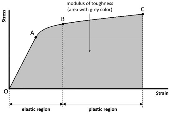
Figure 4. The modulus of toughness is the amount of energy per unit volume necessary to completely break the sample, and is quantified by the area under the entire stress–strain curve.

(9) Modulus of elasticity:

The modulus of elasticity is the slope of the first linear curve, and it is a parameter used to quantify how stiff the sample is within the elastic region. The greater the modulus of elasticity, the stiffer the sample and the greater the resistance to loading within the elastic region.

(10) Tangent modulus:

The tangent modulus is the slope of the second linear curve, and it is a parameter used to quantify how stiff the sample is within the plastic region. The greater the tangent modulus, the stiffer the sample and the greater the resistance to loading within the plastic region. The term “hardening” is used to indicate the phenomenon that the stress increases with the increasing strain within the plastic region. Therefore, the tangent modulus is also called the strain-hardening modulus, used to quantify the degree of hardening. The greater the tangent modulus, the greater the degree of hardening. The tangent modulus must be smaller than the modulus of elasticity, and could be zero. If the tangent modulus is zero (i.e., the second linear curve is horizontal), the plastic property of the material is said to be perfectly plastic.

(11) Strain hardening parameter:

In addition to using the tangent modulus to quantify the degree of hardening, there is another parameter called the strain ha

rdening parameter that can be used to quantify the degree of hardening. The strain hardening parameter is defined as:

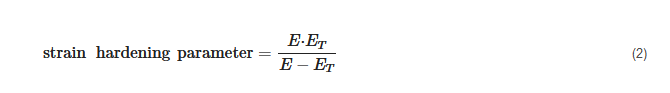
where E is the modulus of elasticity, and ET is the tangent modulus. The greater the strain hardening parameter, the greater the degree of hardening. If ET is equal to E, the strain hardening parameter approaches infinity; however, this case cannot happen in reality, since the tangent modulus must be smaller than the modulus of elasticity. If ET is equal to zero, the strain hardening parameter is equal to zero, and this corresponds to the case that the plastic property of the material is perfectly plastic.

The eleven parameters introduced above can be used to quantify the mechanical properties of any material having a bilinear stress–strain curve, including those of compact bone. In this article, a MATLAB (Mathworks, Natick, MA, USA) computer programming code for analyzing the bilinear stress–strain curve for quantifying these eleven mechanical properties is provided. The readers can use this computer code to analyze these eleven mechanical properties of any material having a bilinear stress–strain curve, including compact bone. Please see the Appendix A for the link to download the computer code and relevant information. Figure 5 shows an example of the analysis result using this computer code. The data shown in Figure 5, adapted from FIGURE 1-19 in ^[11], is a stress–strain curve of a compact bone sample measured using uniaxial tensile test until failure. This data is provided along with the computer code, serving as an example data for the readers to use the computer code.

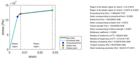
Figure 5. Illustration of an example of the analysis result using the MATLAB computer programming code provided along with this article. By analyzing the bilinear stress–strain curve of a material using this computer code, the associated mechanical properties can be quantified.

References

Tortora, G.J.; Derrickson, B.H. Introduction to the Human Body, 10th ed.; John Wiley & Sons: Hoboken, NJ, USA, 2014.
Nordin, M.; Frankel, V.H. Basic Biomechanics of the Musculoskeletal System, 4th ed.; Lippincott Williams & Wilkins: Philadelphia, PA, USA, 2012.
Çehreli, M. Biomechanics of Dental Implants: Handbook of Researchers; Nova Science: Hauppauge, NY, USA, 2012.
Carter, D.R.; Spengler, D.M. Mechanical properties and composition of cortical bone. Clin. Orthop. Relat. Res. 1978, 135, 192–217.
Kopperdahl, D.L.; Keaveny, T.M. Yield strain behavior of trabecular bone. J. Biomech. 1998, 31, 601–608.
Weiner, S.; Wagner, H.D. The material bone: Structure-mechanical function relations. Annu. Rev. Mater. Sci. 1998, 28, 271–298.
Currey, J.D. How well are bones designed to resist fracture? J. Bone Miner. Res. 2003, 18, 591–598.
Hart, N.H.; Nimphius, S.; Rantalainen, T.; Ireland, A.; Siafarikas, A.; Newton, R.U. Mechanical basis of bone strength: Influence of bone material, bone structure and muscle action. J. Musculoskelet. Neuronal Interact. 2017, 17, 114.
Goodno, B.J.; Gere, J.M. Mechanics of Materials, 9th ed.; Cengage Learning: Boston, MA, USA, 2017.
Turner, C.H. Bone strength: Current concepts. Ann. N. Y. Acad. Sci. 2006, 1068, 429–446.
Marcus, R.; Feldman, D.; Nelson, D.; Rosen, C.R. Fundamentals of Osteoporosis, 4th ed.; Academic Press: London, UK, 2010.

© Text is available under the terms and conditions of the Creative Commons Attribution (CC BY) license; additional terms may apply. By using this site, you agree to the Terms and Conditions and Privacy Policy.

Upload a video for this entry

Information

Subjects: Orthopedics

Contributor MDPI registered users' name will be linked to their SciProfiles pages. To register with us, please refer to https://encyclopedia.pub/register :

Che-Yu Lin

View Times: 3.2K

Update Date: 13 Sep 2021

Table of Contents

Video Upload Options

Confirm

1. Composition and Structure of Bone Tissue

2. Mechanical Properties of Compact Bone

References