 +1 credit
| Version | Summary | Created by | Modification | Content Size | Created at | Operation |
|---|---|---|---|---|---|---|
| 1 | Dr. Costas Sachpazis | + 9036 word(s) | 9036 | 2019-10-06 16:16:30 | | | |
| 2 | Catherine Yang | + 8524 word(s) | 8524 | 2019-10-23 10:37:46 | | | | |
| 3 | Vivi Li | -860 word(s) | 7664 | 2020-10-30 06:59:23 | | |
Video Upload Options
Evaluating the stability of slopes in soil is an important, interesting, and challenging aspect of civil engineering. Despite the advances that have been made, evaluating the stability of slopes remains a challenge. Slope failures are often caused by processes that increase shear stresses or decrease shear strengths of the soil mass [4, 9]. Water plays a role in many of the processes that reduce strength; water is also involved in many types of loads on slopes that increase shear stresses. Another factor involved in most slope failures is the presence of soils that contain clay minerals. In concept, any slope with a factor of safety above 1.0 should be stable [6, 10]. In practice, however, the level of stability is seldom considered acceptable unless the factor of safety is significantly greater than 1.0. In this study an attempt has been done to perform stability analyses corresponding to several different conditions, reflecting different stages in the life of the new railway embankment found in Ethiopia. As various parameters are involved and determined based on correlations, the probabilistic approach was employed to scrutinize the effects of uncertainty on the likelihood of failure. There is no problem with performing a single analysis in which the embankment is considered to be drained and is treated in terms of effective stresses, and in which the clay foundation material is considered to be undrained and is treated in terms of total stresses (during end-of-construction analysis). This is because equilibrium in terms of total stresses must be satisfied for both total and effective stress analyses [2]. The inertia slope stability analysis was used. Since the foundation materials are overconsolidated cohesive soils such as stiff to very stiff clays that tend to dilate during the seismic shaking. The embankment is also expected to be well graded compacted granular material [12]. The critical factor of safety for the railway embankment during short term analysis was found to be 2.199. However, it has increased by 17.6% during the long term analysis (i.e., 2.585). Typical minimum factor of safety used in slope design are about 1.5 for normal long-term loading conditions and about 1.3 for end-of- construction conditions. Apart from that, the minimum short term and long term factor of safety were reduced by 44.5% and 35.9% respectively, due to the introduction of the horizontal seismic load in the limit equilibrium analysis. According to Hynes-Griffin and Franklin (1984) criteria [8] the minimum factor of safety for ~1m tolerable displacement is 1. However, the minimum factor of safety during the pseudostatic analysis (i.e., 1.221) was found to be 22% higher than the required minimum factor of safety. Beside, Newmark’s deformation analysis has been done to predict slope displacement. However, the analysis predicted zero permanent slope displacement. Since; the Newmark (1965) method assumes no deformation of the slope during the earthquake if the pseudostatic factor of safety is greater than 1.0. The more realistic probability of failure is likely in between of 0% and 6.9 %. The sensitivity analysis showed that, the cohesion of the clay layer (i.e., layer II) governs the stability of the railway embankment.
Introduction
The need to move goods and raw materials cheaply, over long distances and often through difficult ground, led to the development of railways. Ultimately, all the loads (static and dynamic) placed on the track by trains are carried by the subgrade. When the subgrade is in the shape of a raised bank constructed above the natural ground, it is called an embankment. The formation at a level below the natural ground is called a cutting. In general terms, the failure of the track bed may be defined as its inability to maintain line and level. The causes of failures can be related to subgrade type, groundwater condition, depth of construction, loading, and speed, among other factors [[1][2], ]. The side slopes of both the embankment and the cutting depend upon the shearing strength of the soil and its angle of repose[3]. The stability of the slope is generally determined by the slip circle method [4].
Evaluating the stability of slopes in soil is an important, interesting, and challenging aspect of civil engineering. Despite the advances that have been made, evaluating the stability of slopes remains a challenge. Even when geology and soil conditions have been evaluated in keeping with the standards of good practice, and stability has been evaluated using procedures that have been effective in previous projects; it is possible that surprises are in store[5]. It is important to understand the agents of instability in slopes for two reasons. First, for purposes of designing and constructing new slopes, it is important to be able to anticipate the changes in the properties of the soil within the slope that may occur over time and the various loading and seepage conditions to which the slope will be subjected over the course of its life. Second, for purposes of repairing failed slopes, it is important to understand the essential elements of the situation that lead to its failure, so that repetition of the failure can be avoided[5] . Slope failures are often caused by processes that increase shear stresses or decrease shear strengths of the soil mass [6]. Water plays a role in many of the processes that reduce strength, water is also involved in many types of loads on slopes that increase shear stresses [[7],[8] ]. It is not surprising; therefore, that virtually every slope failure involves the destabilizing effects of water in some way, and often in more than one way. Another factor involved in most slope failures is the presence of soils that contain clay minerals[8] . The behavior of clayey soils is much more complicated than the behavior of sands, gravels, and non plastic silts, which consist of chemically inert particles [5]. The mechanical behavior of clays is affected by the physicochemical interaction between clay particles, the water that fills the voids between the particles, and the ions in the water. The larger the content of clay minerals, and the more active the clay mineral, the greater is its potential for swelling, creep, strain softening and changes in behavior due to physicochemical effects. Variations of the loads acting on slopes, and variations of shear strengths with time, result in changes in the factors of safety of slopes. As a consequence, it is often necessary to perform stability analyses corresponding to several different conditions, reflecting different stages in the life of a slope [5].
In concept, any slope with a factor of safety above 1.0 should be stable [9]. In practice, however, the level of stability is seldom considered acceptable unless the factor of safety is significantly greater than 1.0. Criteria for acceptable factors of safety recognize (1) uncertainty in the accuracy with which the slope stability analysis represents the actual mechanism of failure, (2) uncertainty in the accuracy with which the input parameters (shear strength, groundwater conditions, slope geometry, etc.) are known, (3) the likelihood and duration of exposure to various types of external loading, and (4) the potential consequences of slope failure. Typical minimum factor of safety used in slope design are about 1.5 for normal long-term loading conditions and about 1.3 for temporary slopes or end-of-construction conditions in permanent slopes [9]. This is because uncertainty and risk are central features of geotechnical and geological engineering. Engineers can deal with uncertainty by ignoring it, by being conservative, by using the observational method, or by quantifying it. In recent years, reliability analysis and probabilistic methods have found wide application in geotechnical engineering and related fields. A central problem facing the geotechnical engineer is to establish the properties of soils and rocks that will be used in analysis, whether that analysis is probabilistic or deterministic [10].
In this study an attempt has been done to perform stability analyses corresponding to several different conditions, reflecting different stages in the life of the new railway embankment found in Ethiopia. As various parameters are involved and determined based on correlations, the probabilistic approach was employed to scrutinize the effects of uncertainty on the likelihood of failure.
Description of site
Project Location and Site Geology
Project Location
Awash – Kombolcha – Hara Gebaya Railway Project (Figure 1) is a 390 km long railway between cities of Awash (km 0), Kombolcha (~km 270) and Hara Gebaya (~km 390). Currently, this railway project is under construction. In this paper, a particular high fill railway embankment at Km 261+140 was chosen for the stability analyses. The approximate elevations along the route (centerline), start with 1821 m at km 260+000, rise to 1836 m at km 261+250 (start of rock protrusion through which tunnel T-07 will be driven), to 1862 m immediately after the tunnel, then to 1915 m at km 263+800[11] . The typical railway embankment under consideration is located in close proximity to kombolcha city. Kombolcha city is a city found in Amhara, Ethiopia. It is located 11.08 latitude and 39.74 longitudes and it is situated at elevation 1883 meters above sea level.
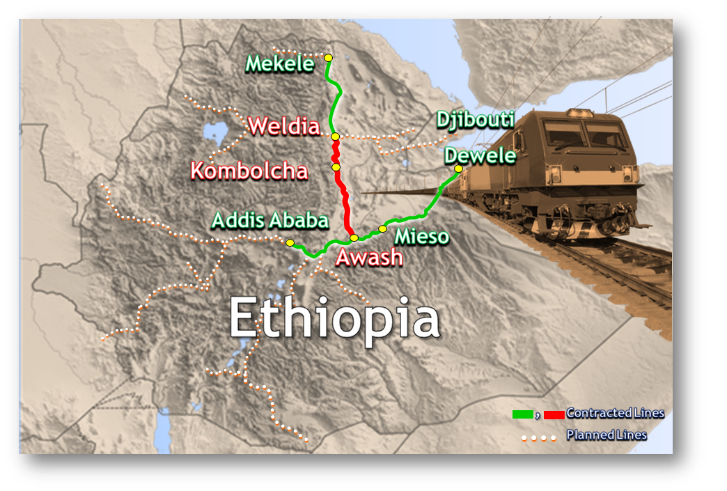
Figure 1: Awash – Kombolcha – Hara Gebaya railway project[11]
Site Geology
The embankment is mainly laid on ancient alluvium (Quaternary lacustrine soil deposits), which is mostly composed of cohesive soils underlain by Ashangi formation. Figure 2a shows the geological map of Ethiopia [12] and figure 2b clearly shows the geological profile along the study area[11] .
 Figure 2a: Geological map of Ethiopia[12]
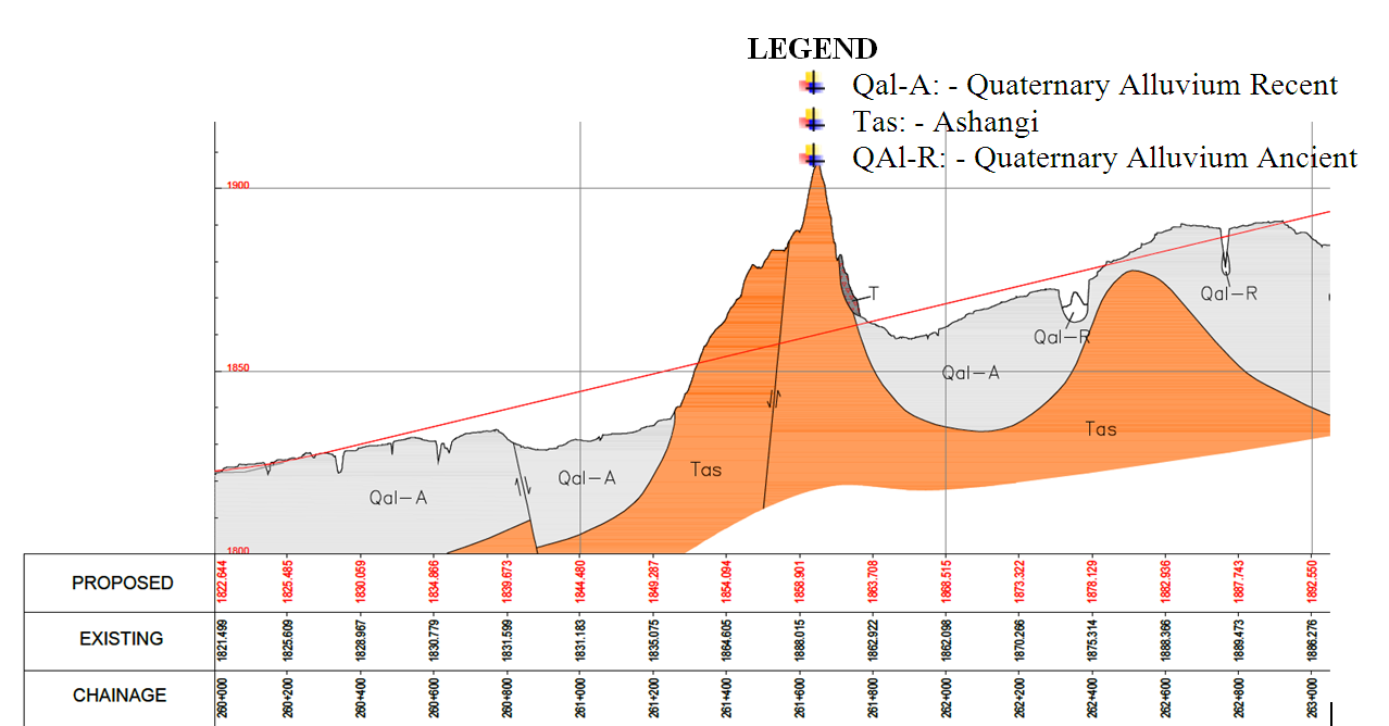
Figure 2b: Geological profile of the proposed railway route along Km 260+000 to 263+000[11]
Soil Properties
Subsurface investigation can include excavation and mapping of test pits and trenches, boring and sampling, in situ testing, and geophysical testing. Such investigations can reveal the depth, thickness, density, strength, and deformation characteristics of subsurface units, and the depth and variation of the ground water table. Laboratory tests are often used to quantify the physical characteristics of the various subsurface materials for input into a numerical slope stability analysis[9] . The required geotechnical properties of the embankment and foundation materials (Table 1) were adopted from the geotechnical report of Awash – Kombolcha – Hara Gebaya Railway Project [11]. The soil strata at Km 261+140 represents ancient lacustrine alluvium and are mainly composed of overconsolidated cohesive soils ranging from stiff to very stiff clay soils. The groundwater table was determined by means of extrapolation from the nearby boreholes and it was found to be 11 m below the ground surface. The expected surcharge load (i.e., 15 kPa) was taken from the report[11] .
Table 1: Geotechnical properties of the railway embankment[11]
|
|
Fill |
Silty clay (layer I) |
Silty clay (layer II) |
Silty clay (layer III) |
Rock |
|
Thickness (m) |
14 |
2 |
11.5 |
8.1 |
8.4 |
|
unsaturated (kN/m3) |
20 |
18 |
18 |
18 |
20 |
|
saturated (kN/m3) |
20 |
18 |
18 |
18 |
20 |
|
E (kPa) |
50,000 |
15000 |
17000 |
25000 |
300000 |
|
0.25 |
0.35 |
0.35 |
0.35 |
0.25 |
|
|
Cu (kPa) |
- |
100 |
100 |
100 |
- |
|
C (kPa) |
0 |
20 |
20 |
20 |
20 |
|
40 |
26 |
26 |
26 |
42 |
|
|
K (m/day) |
8.64 |
0.864E-3 |
8.64E-3 |
8.64E-3 |
0.864 |
|
(m2/year) |
- |
31.54 |
31.54 |
31.54 |
- |
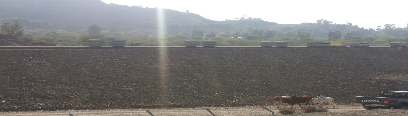
Figure 3: The rail way embankment under construction (Feb, 2016)
Although there is no specific seismic survey performed at Km 261+140, the results obtained from sites (at Km 261+419-261+726 and Km 263+800-263+823) within the same geologic unit and with similar degree of weathering and fracturing/ or similar geotechnical properties have been used. In the absence of site-specific measurement, shear wave velocity (Vs) can be estimated based on correlations with surface geology, in situ-penetration tests, and undrained shear strength may be used, recognizing that these indirect methods introduce greater uncertainty[13] .
- Km 261+419-261+726
(b) Km 263+800-263+823
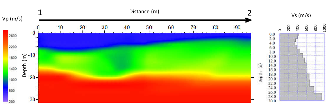
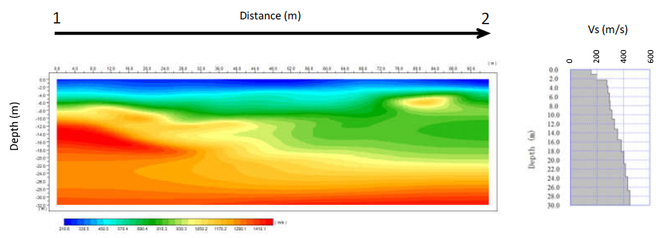
Figure 4: P-wave velocity-depth section and shear wave velocity-depth graph
Seismicity of the Area
The East African Rift system (EARS) is a 3,000-km-long Cenozoic age continental rift extending from the Afar triple junction, between the horn of Africa and the Middle East, to western Mozambique. Seismicity in the East African Rift is widespread, but displays a distinct pattern. Seismicity is characterized by mainly shallow (<40 km) normal faults (earthquakes rupturing as a direct result of extension of the crust), and volcano-tectonic earthquakes[14] . The majority of events occur in the 10–25km depth range. The three limbs of the Afar triple junction zone experience major earthquakes, as well as frequent volcanic eruptions and dike intrusions[15]. In 1961, from the end of May until September, over 3500 earthquakes of magnitude greater than 3.5 shook central Ethiopia[16] . The village of Majete was completely destroyed; in the near town of Kara Kore most masonry houses collapsed. Cracks, fissures and subsidence of up to 1m deep developed on the Addis Ababa-Asmara highway; many culverts and retaining walls along the road had to be rebuilt.
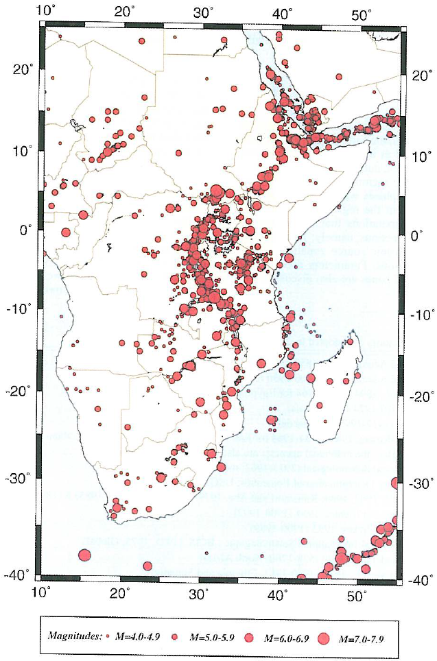
Figure 5a: Seismicity of Eastern & Southern Africa[14] . Earthquake epicenters for Ms > 4.0.
The maximum magnitude reported was 6.6. Reports from outside the epicentral zone in Kombolcha and Dessie, some 60Km north of the actual seismic zone, the tremors were very strong. Later, earth tremors, intensity V were felt in Kombolcha and Dessie during the night of December 1974. Similarly, on 8 July 1977 an earthquake of magnitude 5.0 occurred near the city of Dessie. The USGS indicated a focal depth of 37.6Km[16] . The main shock triggered a landslide along the slope on which Dessie was built. The causalities in Dessie exemplify the need for planning the selection of a site. The distance between Dessie and Kombolcha is about 24Km.
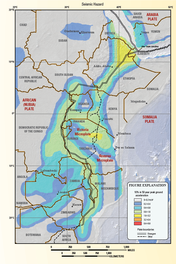
Figure 5b: Seismic hazard of East African regions [15]
Deterministic Slope Stability Evaluation Procedures
Static Slope Stability Analysis
Slopes become unstable when the shear stresses required to maintain equilibrium reach or exceed the available shearing resistance on some potential failure surface. For slopes in which the shear stresses required to maintain equilibrium under static gravitational loading are high, the additional dynamic stresses needed to produce instability may be low. Currently, the most commonly used methods of static slope stability analysis are limit equilibrium analyses and stress-deformation analyses[9] .
Limit Equilibrium Analysis
Limit equilibrium analyses consider force and/ or moment equilibrium of a mass of soil above a potential failure surface. The soil above the potential failure surface is assumed to be rigid (i.e., shearing can occur only on the potential failure surface). The available shear strength is assumed to be mobilized at the same rate at all points on the potential failure surface. As a result, the factor of safety is constant over the entire failure surface. Because the soil on the potential failure surface is assumed to be rigid-perfectly plastic, limit equilibrium analyses provide no information on slope deformations. The factor of safety is a ratio of capacity (the shear strength of the soil) to demand (the shear stress induced on the potential failure surface). In contrast to the assumptions of limit equilibrium analysis, the strength of the soil in actual slopes is not reached at the same time at all points on the failure surface (i.e., the local factor of safety is not constant) [9]. Nearly all limit equilibrium methods are susceptible to numerical problems under certain conditions. These conditions vary for different methods but are most commonly encountered where soils with high cohesive strength are present at the top of a slope and / or when failure surfaces emerge steeply at the base of slopes in soils with high frictional strength [5].
Stress Deformation Analysis
Stress-deformation analyses allow consideration of the stress-strain behavior of soil and rock and are most commonly performed using the finite-element method. For static slope stability analysis, stress-deformation analyses offer the advantages of being able to identify the most likely mode of failure by predicting slope deformations up to (and in some cases beyond) the point of failure, of locating the most critically stressed zones within a slope, and of predicting the effects of slope failures. The accuracy of stress-deformation analyses is strongly influenced by the accuracy with which the stress-strain model represents actual material behavior. The accuracy of simple models is usually limited to certain ranges of strain and / or certain stress paths. Models that can be applied to more general stress and strain conditions are often quite complex and may require a large number of input parameters whose values can be difficult to determine [9].
Analysis Conditions for Static Load Case
End-of-Construction Stability
Slope stability during and at the end of construction is analyzed using either drained or undrained strengths, depending on the permeability of the soil. Many fine grained soils are sufficiently impermeable that little drainage occurs during construction. This is particularly true for clays. For these fine-grained soils, undrained shear strengths are used, and the shear strength is characterized using total stresses. For soils that drain freely, drained strengths are used; shear strengths are expressed in terms of effective stresses, and pore water pressures are defined based on either water table information or an appropriate seepage analysis. The difference between undrained and drained, as these words are used in soil mechanics, is time [5]. Every mass of soil has characteristics that determine how long is required for transition from an undrained to a drained condition. A practical measure of this time is t99, the time required to achieve 99% of the equilibrium volume change, which for practical purposes, is considered to be in equilibrium. Using Terzaghi’s theory of consolidation, one can roughly estimate the value of t99[5]:
(1)
Where t99 is the time required for 99% of the equilibrium volume change, D the greatest distance that water must travel to flow out of the soil mass (length units), and the coefficient of consolidation (length squared per unit of time). For this particular railway embankment, the clay deposits (~21.6m) are sandwiched by relatively permeable materials (Table 1). Hence, it’s worth to consider double drainage condition (i.e., D=21.6/2). From Table 1 the value of is to be 31.54 m/ year. The result obtained by using Equation 1 showed that the condition for 99% of the equilibrium will take approximately 15 years. However, the construction of the embankment is expected to be completed within 80 days[13] . In the mean time, the surcharge loading is expected to occur shortly after construction, the undrained strengths would be the same as those used for end-of-construction stability. Therefore, it was logical to consider undrained condition for the clay soils (using undrained shear strength and total unit weight) and drained conditions for the other materials (using drained shear strength and total unit weight). Undrained strengths for some soils and drained strengths for others can be used in the same analysis [5]. There is no problem with performing a single analysis in which the embankment is considered to be drained and is treated in terms of effective stresses, and in which the clay foundation material is considered to be undrained and is treated in terms of total stresses. Since equilibrium in terms of total stresses must be satisfied for both total and effective stress analyses.
Long-Term Analyses
After a period of time, the clay foundation would reach a drained condition, and the analysis for this condition could be performed using drained Conditions (with effective strength and total unit weight). Because long term and drained conditions carry exactly the same meaning. Both of these terms refer to the condition where drainage equilibrium has been reached and there are no excess pore pressures due to external loads [5]. For the long-term condition, the embankment, clay foundation and the base rock were characterized in terms of effective stresses.
Seismic Slope Stability Analysis
For the seismic evaluation of slope stability, the analysis can be grouped into two general categories, as follows[17]:
Inertia slope stability analysis: The inertia slope stability analysis is preferred for those materials that retain their shear strength during the earthquake. There are many different types of inertia slope stability analyses, and two of the most commonly used are the pseudostatic approach and the Newmark method (1965).
Weakening slope stability analysis: The weakening slope stability analysis is preferred for those materials that will experience a significant reduction in shear strength during the earthquake.
In this study, the inertia slope stability analysis was used. Since the foundation materials are overconsolidated cohesive Soils such as stiff to very stiff clays that tend to dilate during the seismic shaking. The embankment is also expected to be well graded compacted granular material[11] .
Pseudostatic Analysis
The original application of the pseudostatic method has been credited to Terzaghi (1950). This method ignores the cyclic nature of the earthquake and treats it as if it applied an additional static force upon the slope. In particular, the pseudostatic approach is to apply lateral force acting through the centroid of the sliding mass, acting in and out-of-slope direction [17]. The pseudostatic lateral force Fh is calculated by using the following equation,
Fh= khW (2)
Where Fh horizontal pseudostatic force acting through the centroid of sliding mass, in and out-of slope direction, lb or kN. For slope stability analysis, slope is usually assumed to have a unit length (i.e., two-dimensional analysis). Kh is the seismic coefficient, also known as pseudostatic coefficient (dimensionless).
An earthquake could subject the sliding mass to both vertical and horizontal pseudostatic forces. However, the vertical force is usually ignored in the standard pseudostatic analysis. This is because it reduces (increases, depending on its direction) both the driving force and the resisting force [9]. In addition, most earthquakes produce a peak vertical acceleration that is less than the peak horizontal acceleration[17] .
The results of pseudostatic analyses are critically dependent on the value of the seismic coefficient, Kh. selection of an appropriate pseudostatic coefficient is the most important and most difficult aspect of a pseudostatic stability analysis. There are no hard and fast rules for selection of a pseudostatic coefficient for design. It seems clear, however, that the pseudostatic coefficient should be based on the actual anticipated level of acceleration in the failure mass (including any amplification or deamplification effects) and that it should correspond to some fraction of the anticipated peak acceleration [9]. Although engineering judgment is required for all cases, the criteria of Hynes-Griffin and Franklin (1984) should be appropriate for most slopes. Previous studies regarding to the earthquake coefficients of peak ground acceleration values (PGA) for the Afar area of Ethiopia ranged from 0.1g to o.75g[18] . Considering the previous works and the map compiled by the USGS [15]a peak ground acceleration of 0.3g for 10% probability of occurrence in 50 years was selected for the analysis. Beside, based on the criteria provided by Hynes-Griffin and Franklin (1984); an acceleration multiplier factor of 0.5 and 80% of the static shear strength were used during the pseudostatic analyses.
However, representation of the complex, transient, dynamic effects of the earthquake shaking by a single constant unidirectional pseudostatic acceleration is obviously quite crude. Experience has clearly shown, for example, that, pseudostatic analyses can be unreliable for soils that build up large pore pressures or show more than 15% degradation of strength due to earthquake shaking. Pseudostatic analyses produced factors of safety well above 1 for a number of dams that later failed during earthquakes. These cases illustrate the inability of the pseudostatic method to reliably evaluate the stability of slopes susceptible to weakening instability[9] .
Apart from its limitation, the analysis is relatively simple and straightforward; indeed, its similarity to the static limit equilibrium analyses routinely conducted by geotechnical engineers makes its computations easy to understand and perform. It produces a scalar index of stability (the factor of safety) that is analogous to that produced by static stability analyses. Many commercially available computer programs for limit equilibrium slope stability analysis have the option of performing pseudostatic analyses[9] .
Earthquakes Immediately after Construction
Seismic loading is of short duration, it is reasonable to assume that except for some coarse gravels and cobbles, the soil will not drain appreciably during the period of earthquake shaking. Pseudostatic analyses for short-term stability are only appropriate for new slopes [5]. In this case, stability computations were performed by using undrained shear strengths that reflect the effects of cyclic loading for low-permeability materials; effective stresses and drained shear strengths were used for high-permeability soils.
Earthquakes After the Slope Has Reached Consolidated Equilibrium
Here, the slope stability computations were performed by using a two-stage analysis procedure. A first-stage analysis was performed for conditions prior to the earthquake (no seismic coefficient) to compute effective stresses at the base of each slice. The strengths were computed according to the Mohr-Coulomb strength law and the effective stress strength properties. The resulting effective stress strengths were treated as equivalent undrained strengths in the second stage of the analysis. The simple effective stress approach requires only the conventional effective stress strength properties [5]. The equivalent undrained shear strengths were then used in the second-stage computations (with seismic coefficient) to compute the pseudostatic factor of safety for the slope.
Newmark Method
The pseudostatic method of analysis, like all limit equilibrium methods, provides an index of stability (the factor of safety) but no information on deformations associated with slope failure. Since the serviceability of a slope after an earthquake is controlled by deformations, analyses that predict slope displacements provide a more useful indication of seismic slope stability. In view of the fact that earthquake-induced accelerations vary with time, the pseudostatic factor of safety will vary throughout an earthquake [9]. The purpose of the Newmark (1965) method is to estimate the slope deformation for those cases where the pseudostatic factor of safety is less than 1.0 (i.e., the failure condition)[15]. The Newmark (1965) method assumes that the slope will deform only during those portions of the earthquake when the out-of-slope earthquake forces cause the pseudostatic factor of safety to drop below 1.0. When this occurs, the slope will no longer be stable, and it will be accelerated down slope. The longer that the slope is subjected to pseudostatic factor of safety below 1.0, the greater the slope deformation. On the other hand, if the pseudostatic factor of safety drops below 1.0 for a mere fraction of a second, then the slope deformation will be limited. Obviously, the sliding block model will predict zero permanent slope displacement if earthquake-induced accelerations never exceed the yield acceleration. The yield acceleration is the minimum pseudostatic acceleration required to produce instability of the block[9] .
The effects of slope response on the inertial force acting on a potential failure mass can be computed using dynamic stress-deformation analyses. Using the dynamic finite-element analysis, the horizontal components of the dynamic stresses acting on a potential failure surface are integrated over the failure surface to produce the time-varying resultant force that acts on the potential failure surface. This resultant force can then be divided by the mass of the soil above the potential failure surface to produce the average acceleration of the potential failure mass. Although the procedure was developed originally for dams, the basic concept can be applied to any type of slope. The average acceleration time history (depending on the input motions and the amplification characteristics of the slope), provides the most realistic input motion for a sliding block analysis of the potential failure mass[9] .
Acceleration Time History
A design motion with the desired characteristics can be selected from the strong motion accelerograms that have been recorded during previous earthquakes or from artificially generated accelerograms[19] . From the regional seismic review, earthquakes with magnitude, M greater than 6 can be expected to likely occur in the study area. As there is no recorded accelerograms in/ around the study area, the commonly used acceleration time history, the 1940 Elcentro (California) earthquake is used [20]. The model used for the stability analysis includes the soil layers and a base of bed rock. The appropriate input motion at depth can be computed through a ‘deconvolution’ analysis using a 1-D wave propagation code such as the equivalent-linear program Shake[21] .
The 1940 Elcentro (California) earthquake acceleration time history was scaled to the peak ground acceleration of 0.3g and applied at point A as a base rock motion (Figure 6). Then, the object motion at point B was determined by using a computer program for the 1-D analysis of geotechnical earthquake engineering problems the so-called Shake2000. Since the deconvolution procedure is beyond the scope of this paper, interested readers are suggested to read the following references[19] , [21]and [22].
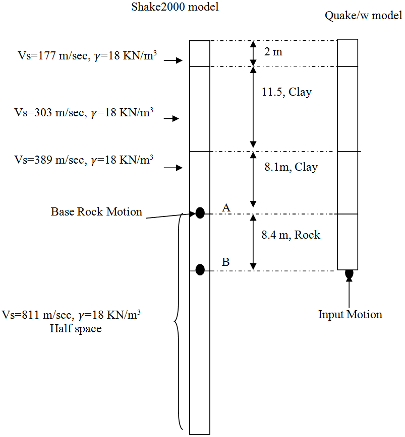
Figure 6: Deconvolution procedure used to determine the input motion
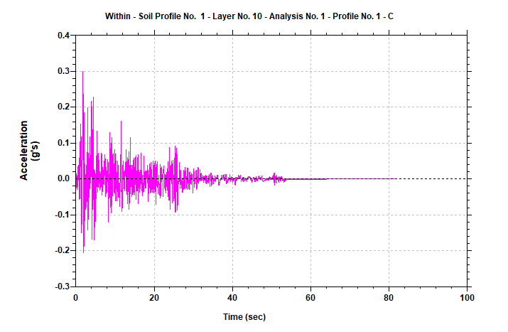
Figure 7: Base rock motion applied at point A
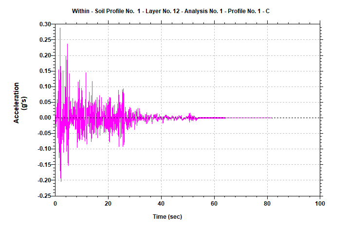
Figure 8: Input motion used for the Quake/w model (obtained from point B)
Probabilistic Stability Evaluation Procedures
The current state of practice relies on using calculated FOS values in the design process to account for uncertainties associated with soil parameters, site stratigraphy, ignorance, and the potential consequences if the slope fails. Under ideal conditions, a FOS of at least 1 should ensure safe design, but because of all the uncertainties, a higher value of the FOS is desirable for design recommendations. Two slopes with the same FOS may have considerably different levels of safety depending on how well the site has been characterized with a view to minimizing uncertainties. To account for such levels of uncertainty, the probabilistic method should be considered for assessing the performance of the slope. Such analysis can take into account uncertainties associated with the site stratigraphy, soil parameters, and even the method of analysis. Of course the final result here will be the probability of failure, or alternatively, the probability of unsatisfactory performance [6].
Many measures of soil strength appear to be well-modeled by Normal distributions, or by more flexible distributions of such as the four-parameter Beta, which mimic the Normal within the high probability density region of the distribution[10] .
Since the mean and the standard deviation values are expressed in the same units, a non-dimensional term can be introduced by taking the ratio of the standard deviation and the mean. This is called the coefficient of variation (COV) for a deterministic variable; COV(X) is zero. A smaller value of the COV indicates a smaller amount of uncertainty or randomness in the variable, and a larger amount indicates a larger amount of uncertainty. In many engineering problems, a COV of 0. 1 to 0.3 is common for a random variable[23] .
Estimates Based on Published Values
In this particular project, some of the values of soil properties were estimated based on correlations or on meager data plus judgment, and it is not possible to calculate values of standard deviation or coefficient of variation based on statistical estimates. Because standard deviations or coefficients of variation are needed for reliability analyses, it is essential that their values can be estimated using experience and judgment. Values of COV for various soil properties and in situ tests are shown in Table 2.
Table 2: COV for soil properties [5]
|
Property or in situ test |
COV (%) |
References |
|
Unit weight ( ) |
3-7 |
Harr (1987), Kulhawy (1992) |
|
Effective stress friction angle |
2-13 |
Harr (1987), Kulhawy (1992), Duncan (2000) |
|
Undrained shear strength |
13-40 |
Kulhawy (1992), Harr (1987), Lacasse and Nadim (1997) |
|
Undrained Vane shear |
10-20 |
Kulhawy (1992) |
The 3 Rule
The rule of thumb [5] uses the fact that 99.73% of all values of a normally distributed parameter fall within three standard deviations of the average. Therefore, if HCV is the highest conceivable value of the parameter and LCV is the lowest conceivable value of the parameter, these are approximately three standard deviations above and below the average value.
(3)
Where HCV is the highest conceivable value of the parameter and LCV is the lowest conceivable value of the parameter. This rule of thumb (Equation 3) has been used to compute the standard deviations as shown in Table 3. Since the minimum factor of safety was obtained during earthquake immediately after construction, further probabilistic stability analysis has been done for this condition to study the effects of uncertainty on the likelihood of failure.
Table 3: Determination of standard deviation based on the 3 rule
|
|
LCV |
HCV |
MLV*
|
COV (%) |
|
|
Embankment ( ) |
25 |
45 |
tan-1(0.8*tan400) = 33.87 |
3.3 |
~10 |
|
Clay foundation (Cu) |
40 |
120 |
0.8*100 = 80 |
13.3 |
~17 |
*most likely value (MLV)
The COVs obtained by using the 3 Rule (Table 3) were in agreement with the published data. Since the main controlling issue there is the strength of the embankment and the clay foundation, the strength of the base rock was considered to be a constant.
A Monte Carlo scheme was used to compute a probability distribution of the resulting safety factors. The study [24]showed that the reliability index ( ) is independent of the seed random number generator and a sample size of 700 or greater is a good choice for Monte Carlo simulation method (MCSM). It has been suggested that the number of required Monte Carlo trials is dependent on the desired level of confidence in the solution, as well as the number of variables being considered. Statistically, the following equation can be developed[25] .
(4)
Where Nmc is number of Monte Carlo trials, is the desired level of confidence (0 to 100%) expressed in decimal form, d is the normal standard deviate corresponding to the level of confidence, and m is number of variables.
Table 4: Normal Standard Deviate
|
Percentage of confidence (%) |
Normal standard deviate (d) |
|
80 |
1.28 |
|
85 |
1.44 |
|
90 |
1.64 |
|
95 |
1.96 |
|
99 |
2.57 |
In fact, for a 100% level of confidence, an infinite number of trials will be required. The number of Monte Carlo trials was determined by using Equation 4 and Table 4. As a result, a sample size of 5,000 (for 90% of confidence) was used in the application of MCSM. Once the probability distribution of the safety factors are known, other quantifying parameters, such as the probability of failure can be determined[25] . All the variables in Table 3 were assumed to have a normal distribution. The corresponding probability distribution functions are shown in Figure 9.
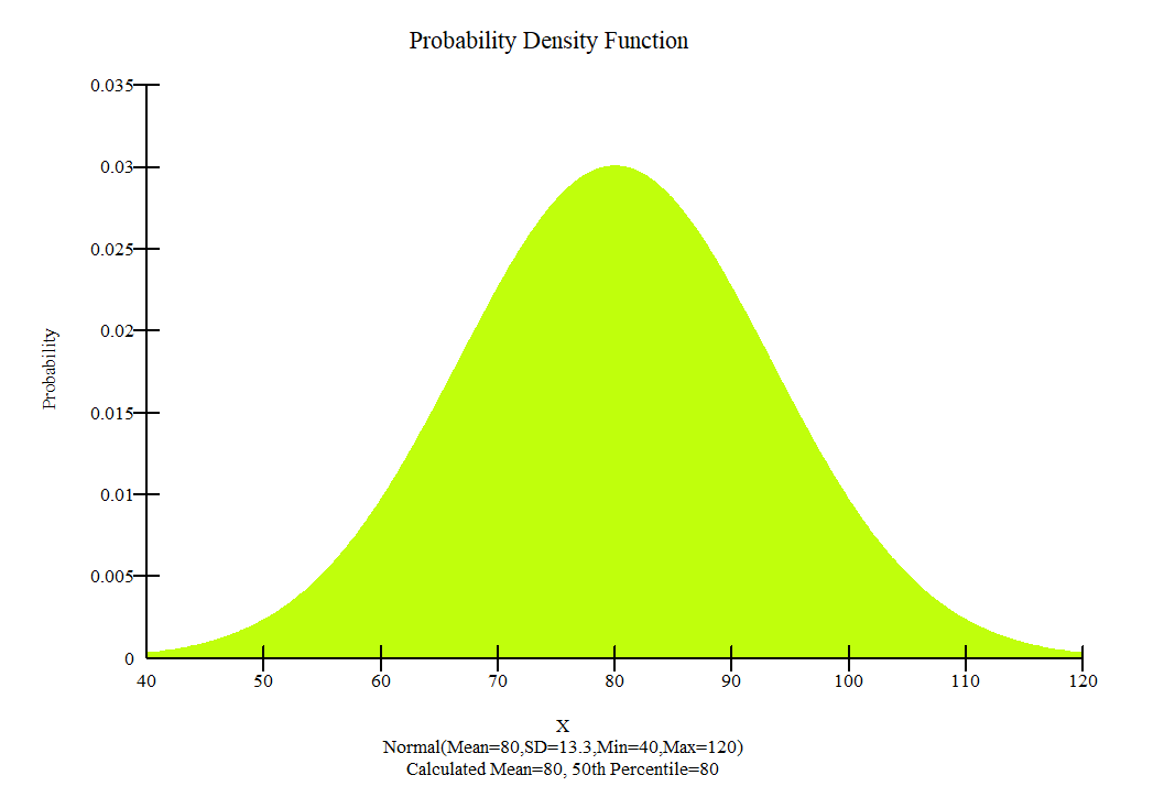
- Clay foundation
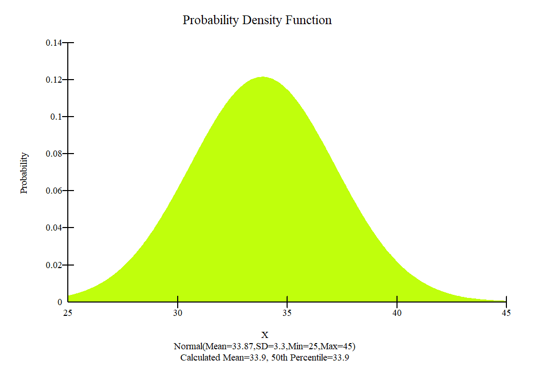
- (b) Embankment
Figure 9: Probability density function used for the embankment and clay foundation
As is well known, many natural data sets follow a bell-shaped distribution and measurements of many random variables appear to come from population frequency distributions that are closely approximated by a normal probability density function. This is also true for many geotechnical engineering material properties. In equation form, the normal probability density function is [25]:
(5)
Where x is the variable of interest, u is the mean, and σ is the standard deviation.
C – Correlation
Correlation between strength parameters may affect the probability distribution of a slope. In this study, a zero correlation coefficient was used (i.e., c and φ are independent parameters).
Spatial Variability
Spatial variability in the soil properties can be an important consideration in certain cases. This is particularly true when the potential slip surface is relatively long within one soil. Sampling the soil only once, and sampling the soil strength for each slice have been applied during the analyses.
Sensitivity Analysis
A sensitivity analysis is somewhat analogous to a probabilistic analysis. Instead of selecting the variable parameters randomly, the parameters were selected in an ordered fashion using a Uniform Probability Distribution function. For presentation purposes, all the strengths were normalized to a value ranging between 0.0 and 1.0. Zero means the lowest value and 1.0 means the highest value. Minimum and maximum values were used as per Table 3.
Software
Slope/w
Analyzing the stability of earth structures is the oldest type of numerical analysis in geotechnical engineering. Modern limit equilibrium software is making it possible to handle ever-increasing complexity within an analysis. It is now possible to deal with complex stratigraphy, highly irregular pore-water pressure conditions, and various linear and nonlinear shear strength models, almost any kind of slip surface shape, concentrated loads, and structural reinforcement[25] . SLOPE/W is one component in a complete suite of geotechnical products called GeoStudio. One of the powerful features of this integrated approach is that it opens the door to types of analyses of a much wider and more complex spectrum of problems, including the use of finite element computed pore-water pressures and stresses in a stability analysis.
In this study slope/w has been employed to determine the factor of safety of the railway embankment. For the analyses mathematically more rigorous formulation (Morgenstern-Price) which includes all interslice forces and satisfies all equations of statics has been chosen. Interestingly, when the cohesion of a soil is specified as zero, the minimum factor of safety will always tend towards the infinite slope case. Moreover, the critical slip surface is parallel and immediately next to the slope face[25] . To get a more realistic slip surface in a SLOPE/W analysis the embankment material was defined with suction parameter, b equal to 20 degrees. Usually, b is greater than zero, but less than ’. Most common values range from 15 to 20 degrees[25] . In addition to this, at the crest, the normal at the base of the first slice will point away from the slice, indicating the presence of tension instead of compression. Generally, this is considered unrealistic, particularly for materials with little or no cohesion. Physically, it may suggest the presence of a tension crack[25] . To capture this phenomenon, an automatic search option for tension crack was selected; also entry and exit method was used to define the slip surface.
SLOPE/W includes a general comprehensive algorithm for probabilistic analyses. Therefore, both the probabilistic and sensitivity analyses have been carried out by using slope /w.
Quake/w
SLOPE/W can use the results from a QUAKE/W dynamic analysis to examine the stability and permanent deformation of earth structures subjected to earthquake shaking using a procedure similar to the Newmark method[26] . QUAKE/W is a finite element program for analyzing the effects of earthquakes on embankments and natural slopes. The software computes the static plus dynamic ground stresses at specified intervals during an earthquake. Most importantly, SLOPE/W can use these stresses to analyze the stability variations during the earthquake and estimate the resulting permanent deformation.
The first step in any QUAKE/W analysis is to establish the in-situ stress state conditions that exist before the earthquake occurs. Because it is necessary to establish the initial static stresses before subjecting the structure to the dynamic action [26]. In QUAKE/W analysis the initial in-situ static stress were computed with the Initial Static analysis type, and equivalent linear material model was chosen. Beside shear modulus reduction functions were determined based on the previous studies [27]and [28] .
Earthquake records often have some vibrating noise at the start of the record and at the end of the record. Altering the input motion record to the bare minimum is effective in mitigating the required computing time. Therefore the input motion shown in Figure 8 was modified to duration of 55 seconds. To properly capture the effects of an earthquake, the time stepping sequence was determined based on the input earthquake record.
Boundary condition for the in-situ stress analysis
Along the vertical ends of the problem, one must specify the equivalent of rollers (Figure 10). This is done by specifying a zero x-displacement condition along these edges. The ground is free to move in the vertical direction, but is fixed in the horizontal direction. In the mean time, the problem is fixed along the base. This is accomplished by specifying the displacement to be zero in both the horizontal (x) and vertical (y) directions.

Figure 10: Boundary conditions for the Initial Static analysis
Dynamic Analysis
Once the in-situ static stresses established, the next step was to do the dynamic or shaking analysis. With the KeyIn Analyses command, a new QUAKE/W analysis was created where the “Parent” is the previous Initial Static analysis. Both the initial stress conditions and the pore-pressure conditions came from the Parent (previous) analysis. The Equivalent Linear Dynamic analysis type was used.
Boundary condition for the Dynamic Analysis
The boundary conditions at the vertical ends of the problem have to be changed for the dynamic analysis. In this case the vertical movement was fixed, but the ground was allowed to move laterally. These conditions allow the ground to sway from side to side when the horizontal earthquake accelerations are applied. Specifying a vertical displacement of zero at the ends is not strictly correct, but the boundary is sufficiently far away from the slope so that the zero displacement boundary doesn’t affect the dynamic shear stresses in the slope[26] .
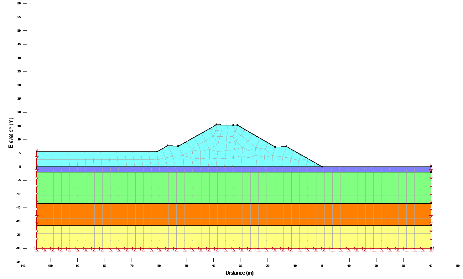
Figure 11: Boundary conditions for the dynamic analysis
Result
Results of stability calculations for each condition (i.e., end-of-construction, earthquake immediately after construction, long-term, earthquake after the slope has reached consolidated equilibrium and Newmark deformation) are presented in separate Figures as shown in Figure 12a,b. The Figures show the most critical slip surface that gave the minimum factor of safety. To save paper space only a typical result for the lower portion of the slope has been included.
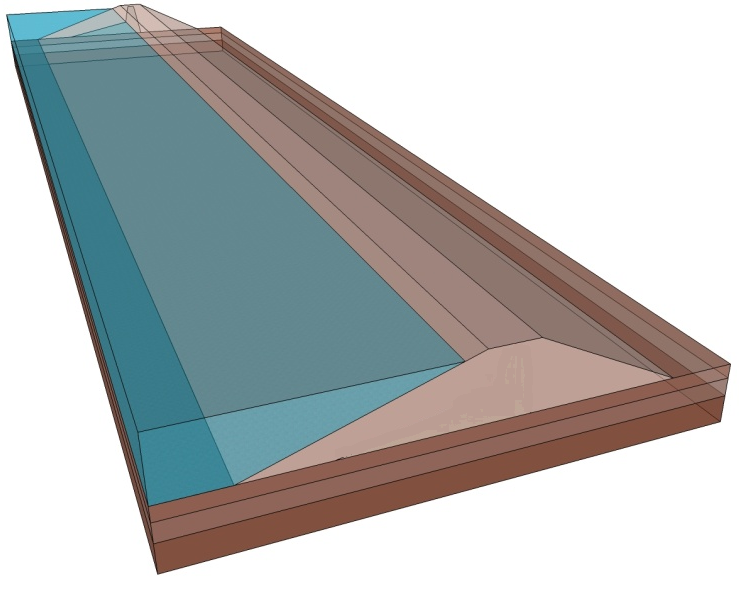
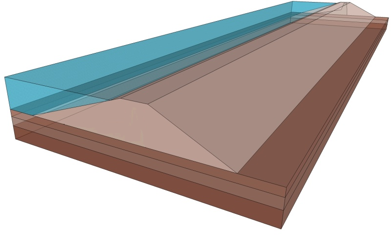
Figure 12a: 3-D Model Views (Block Views) based on dimensions.
- end-of-construction
- earthquake immediately after construction
- long-term
- earthquake after the slope has reached consolidated equilibrium
(e) end-of-construction for the lower portion of the slope
(f) Newmark deformation

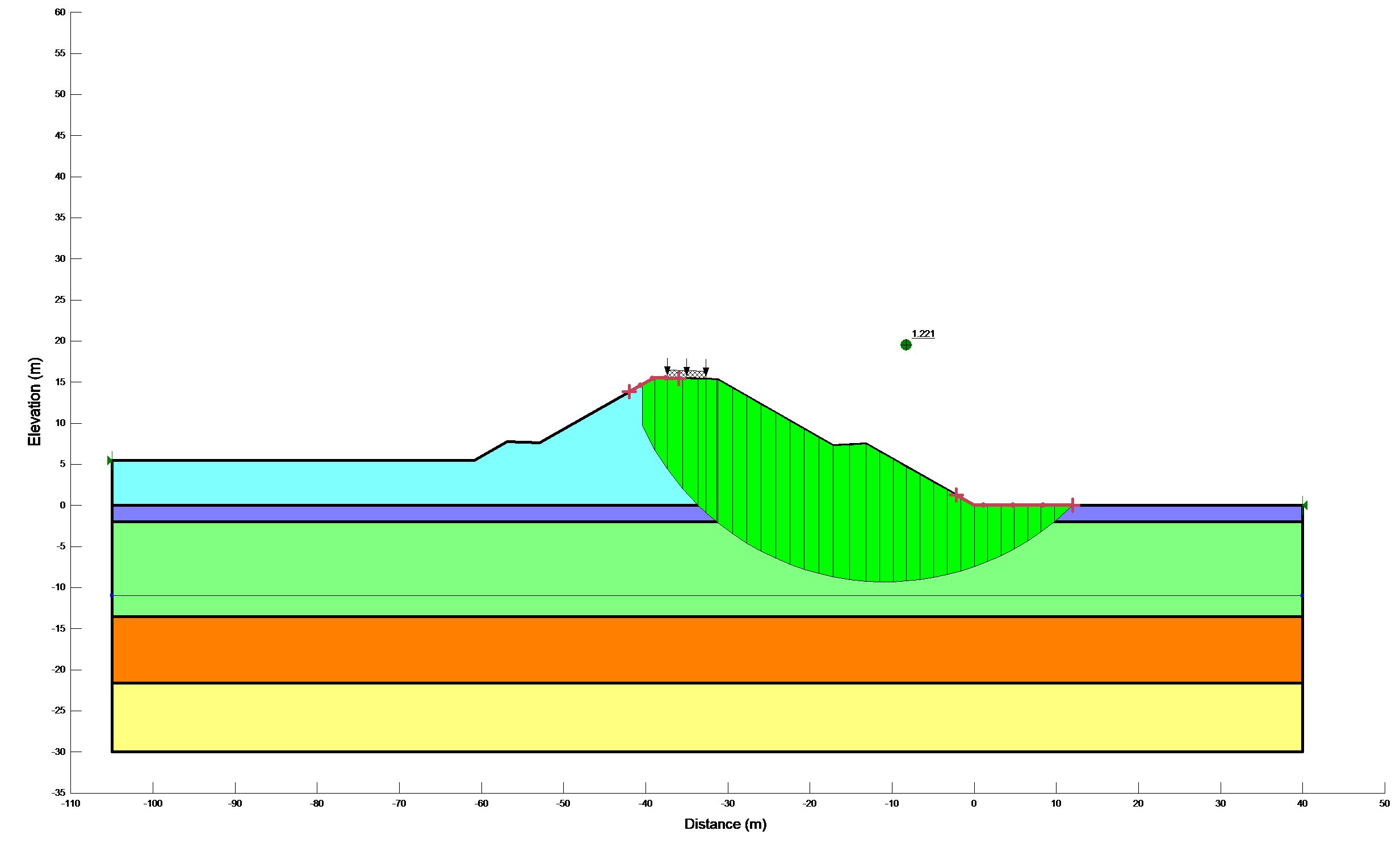
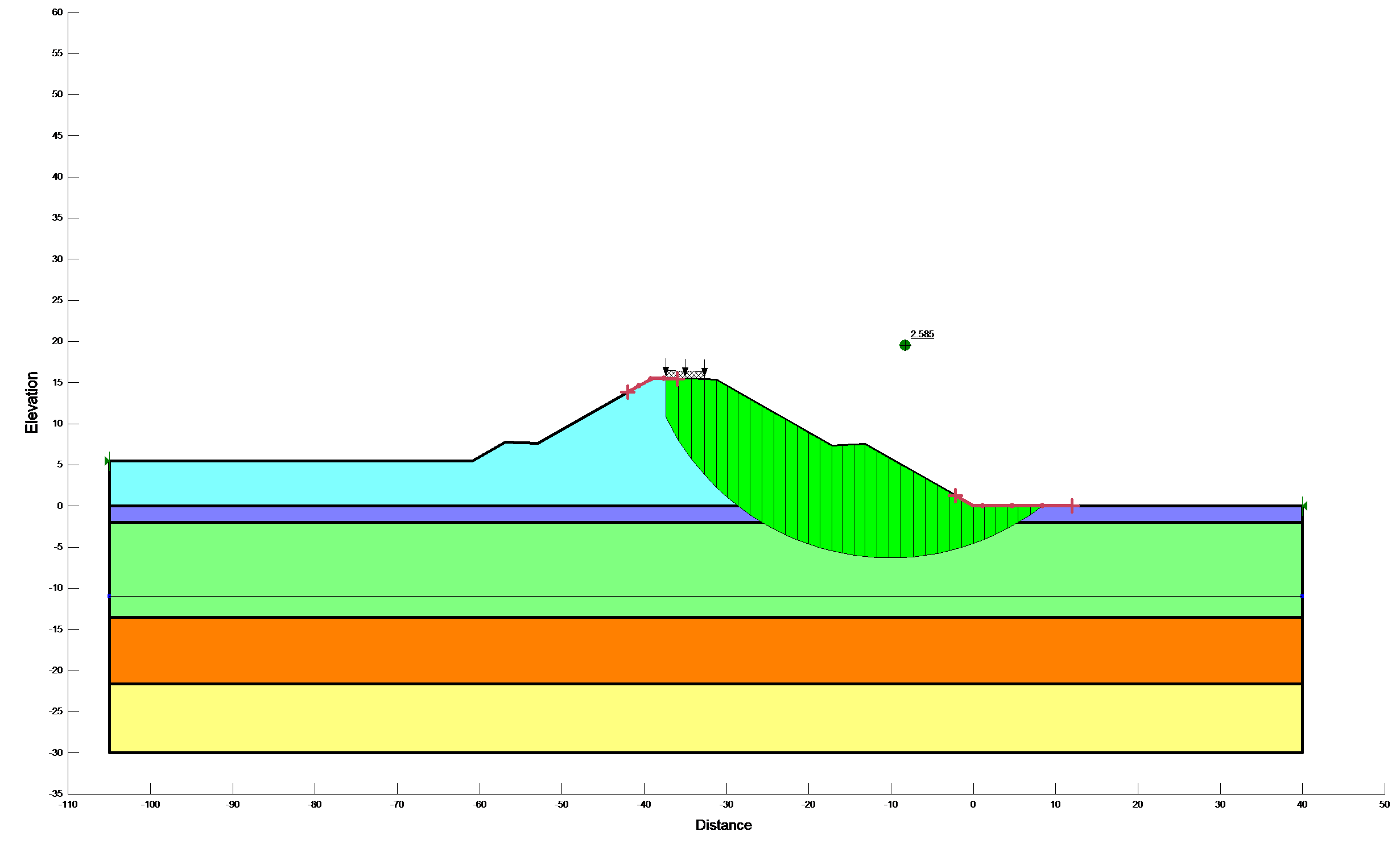

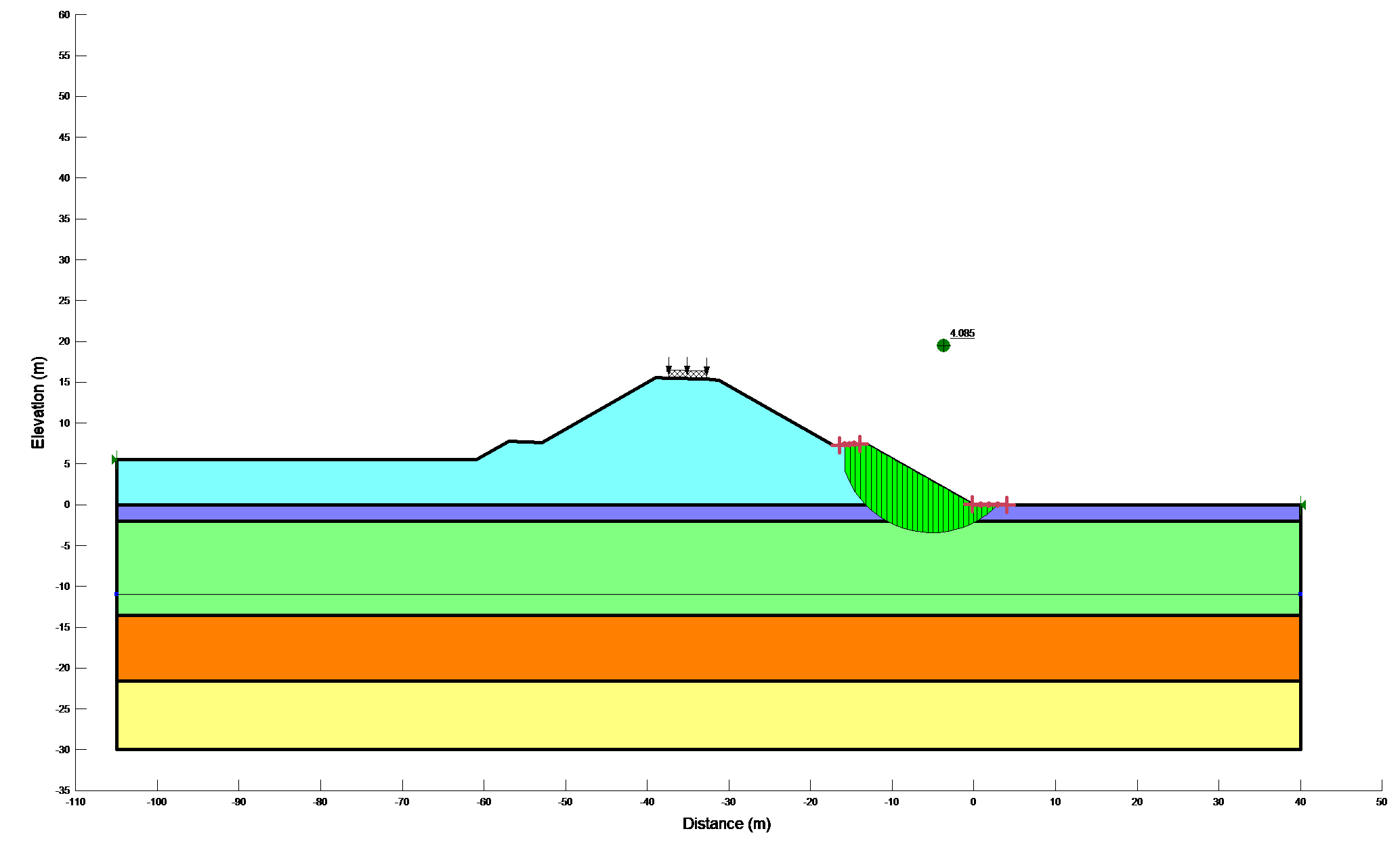

Figure 12b: Results of stability calculations for each condition
The results of deterministic slope stability calculations are summarized and tabulated in Table 5.
Table 5: Summaries of deterministic slope stability calculations
|
Analysis |
Overall slope (F.S.) |
Lower portion of slope (F.S.) |
|
|
Short term |
2.199 |
4.085 |
|
|
Earthquakes before equilibrium |
1.221 |
2.456 |
|
|
Long term |
2.585 |
2.982 |
|
|
Earthquake after equilibrium |
1.656 |
2.013 |
|
|
Using Quake /w results |
1.695 |
2.123 |
|
Figure 13 shows the result obtained from Newmark’s deformation analysis (i.e., the computed factor of safety versus the average acceleration of the slip surface). As expected, the factor of safety was inversely proportional to the average acceleration.
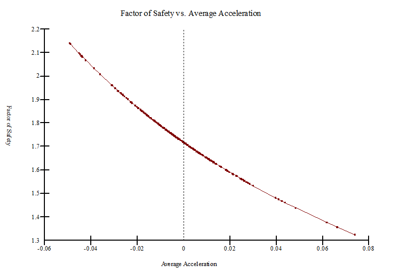
Figure 13: Factor of safety versus average acceleration
A probability density function of the 5,000 computed factors of safety (when sampled only once) is shown in Figure 14. Since the variability of the soil properties is normally distributed, the probability density function of the factor of safety (Figure 14) is also normally distributed as expected. The corresponding statistical parameters are also tabulated in Table 6.
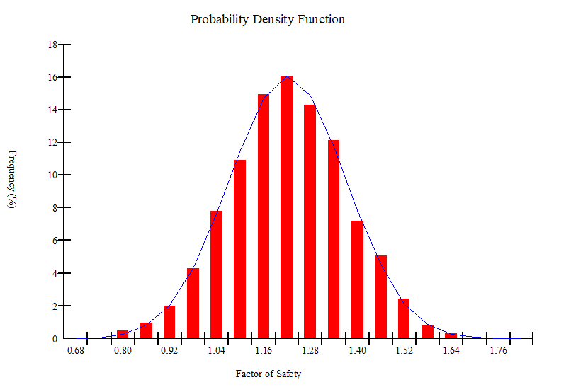
Figure 14: Probability density function of the factor of safety
Table 6: Statistical parameters of the 5,000 computed factors of safety
|
Parameters |
Values |
|
|
Mean F of S |
1.22 |
|
|
Reliability Index |
1.48 |
|
|
P (Failure) (%) |
6.9 |
|
|
Standard deviation |
0.149 |
|
|
Min F of S |
0.72 |
|
|
Max F of S |
1.69 |
|
|
Number of trials |
5,000 |
|
Similarly, Figure 15 shows the probability distribution function of the 5,000 Monte Carlo factors of safety. The red line represents the probability of failure (6.9%). However, when new soil properties sampled for every slice in each Monte Carlo trial the probability of failure was reduced to 0% and the minimum factor of safety was 1.1.
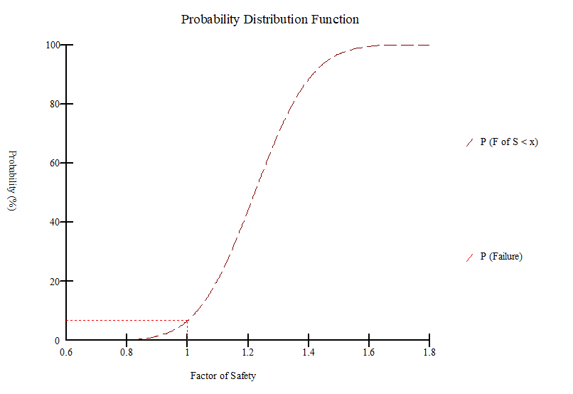
Figure 15: Probability Distribution Function
Finally, a sensitivity graph showing the computed factor of safety at different values of the parameters is shown in Figure 16.
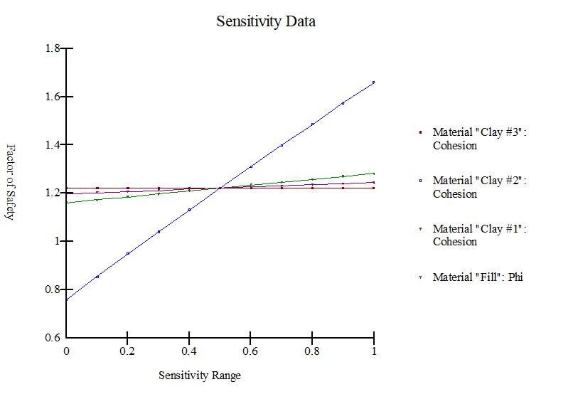
Figure 16: Sensitivity graph
Disussions
As previously mentioned, the clay materials were defined in terms of undrained shear strength parameters and the freely draining materials were defined in terms of effective shear strength parameters during the short term analysis. Considering both drained and undrained shear strength parameters in a single analysis has no problem. This is because equilibrium should be satisfied in terms of total stresses in both cases. The critical factor of safety for the railway embankment during short term analysis was found to be 2.199. However, it has increased by 17.6% during the long term analysis (i.e., 2.585). Typical minimum factor of safety used in slope design are about 1.5 for normal long-term loading conditions and about 1.3 for end-of- construction conditions. Apart from that, the minimum short term and long term factor of safety were reduced by 44.5% and 35.9% respectively, due to the introduction of the horizontal seismic load in the limit equilibrium analysis. These results showed that the horizontal pseudostatic force clearly decreased the factor of safety. Since it reduced the resisting force and increased the driving force. According to Hynes-Griffin and Franklin (1984) criteria [5] the minimum factor of safety for ~1m tolerable displacement is 1. In this study, the minimum factor of safety during the pseudostatic analysis (i.e., 1.221) was found to be 22% higher than the required minimum factor of safety. Since the serviceability of a slope after an earthquake is controlled by deformations, Newmark’s deformation analysis has been done to predict slope displacement. However, the analysis predicted zero permanent slope displacement. This is because; the Newmark (1965) method assumes no deformation of the slope during the earthquake if the pseudostatic factor of safety is greater than 1.0.
SLOPE/W has a general comprehensive algorithm for probabilistic analyses. The Monte Carlo scheme in SLOPE/W involves numerically sampling the statistical variables numerous times. The sampling can be controlled by optionally excluding or including spatial variability in the analysis. When spatial variability was not selected as a consideration in slope/w, all the statistical parameters were sampled before computing the factor of safety and the parameters were consequential constant for each Mote Carlo run. The highest probability of failure (6.9%) occurred when no consideration was given to spatial variability. This is logical since it is possible that all statistical parameters have their lowest values all at the same time. This also results in the lowest possible factor of safety. On the contrary, the lowest probability of failure occurs when sampling the statistical parameters for every slice. In fact the lowest of the 5,000 computed factor of safety was greater than 1(i.e., 1.1), the probability of failure was not existent. This is because properties were sampled too often for one Monte Carlo run; the solution tends towards the mean or overall average conditions. This yielded the lowest probability of failure.
These two options are useful to compute the range of the probability of failure[25] . The more realistic probability of failure is likely in between of 0% and 6.9 %. When more field investigation and soil testing are available, and when more statistical data become available to justify the use of a certain sampling distance, the probability of failure can be more accurately estimated. Unfortunately, sufficient data is seldom available to formally evaluate the spatial variability, and so it comes down to making a judgment. Making an intuitive judgment, however, may be better in some cases than ignoring the possibility of spatial variability completely[25] . The sensitivity analysis showed that the cohesion of the clay layer (i.e., layer II) governed the stability of the railway embankment.
Conclusions
In this study stability analyses were carried out by considering different scenarios, reflecting different stages in the life of the new railway embankment found in Ethiopia. Since, various parameters were determined based on correlations from field test results, the probabilistic approach has been used to analyze the effects of uncertainty on the likelihood of failure. After careful examination of the results, the following conclusions were pointed out.
Among all considered circumstances, the minimum factor of safety (1.221) was obtained, when the analysis considered Earthquakes before equilibrium has reached. The result revealed that the computed pseudostatic factor of safety was greater than the required minimum factor of safety as per Hynes-Griffin and Franklin (1984) criteria. Beside, the superimposed seismic load upon the previously existing static shear stresses, the dynamic shear stresses couldn’t exceeded the available shear strength of the soil and didn’t produce inertial instability of the slope. Also, Newmark’s deformation analysis predicted zero permanent slope displacement. Since, the pseudostatic factor of safety was greater than 1.0.
At 90% confidence level, the highest probability of failure was found to be (6.9%) while no consideration was given to spatial variability. However, the probability of failure was not existent when sampling the statistical parameters for every slice. Therefore, the more realistic probability of failure is likely in between of 0% and 6.9%. One should understand that, the degree of uncertainty in the input parameters may not warrant a high level of confidence in a probabilistic analysis.
References
- Braja M. Das. Geotechnical Engineering Handbook; J. Ross publishing: USA, 2011; pp. 499.
- Sachpazis, C.I. Geotechnical Site Investigation Methodology for Foundation of Structures; Published in the Bulletin of the Public Works Research Centre: Greece, 1988; pp. Edition January - June 1988.
- Sachpazis, C.I. Detailed Slope Stability Analysis and Assessment of the Original Carsington Earth Embankment Dam Failure in the UK; Bund. Z of the Electronic Journal of Geotechnical Engineering : USA, 2013; pp. Volume 18.
- Satish Chandra. Railway Engineering; Oxford University Press: UK, 2007; pp. 585.
- Michael Duncan and Stephen G. Wright, . Soil Strength and Slope Stability; John Wiley & Sons Inc: USA, 2005; pp. 293.
- Abramson, L.W., Lee, T.S., Sharma, S., and Boyce, G.M. Slope Stability and Stabilization Methods; John Wiley & Sons Inc: USA, 2002; pp. pp.712.
- Sachpazis, C.I. (2014), "Experimental Conceptualisation of the Flow Net system construction inside the body of homogeneous Earth
- Sachpazis, C.I. (1989), "Slope Stability Problems in Messochori, Karpathos island". Proceedings of 2nd Conference of the Bulletin of Hellenic Geographical Society.
- Kramer, S.L. Geotechnical Earthquake Engineering; Prentice Hall: USA, 1996; pp. pp. 437.
- John T. Christian; Geotechnical Engineering Reliability: How Well Do We Know What We Are Doing?. Journal of Geotechnical and Geoenvironmental Engineering 2004, 130(10), 985-1003, 10.1061/(ASCE)1090-0241(2004)130:10(985).
- Yapi Merkezi, 2016. Awash – Kombolcha – Hara Gebeya Rail Way Project Alignment Geotechnical Report KM: 260+000-270+500. Yapi Merkezi Ethiopian Branch, pp. 614
- Kazmin, V., (1972), Geological map of Ethiopia, Geological Survey of Ethiopia, Ministry of Mines, Energy and Water Resources, Addis Ababa
- Bernard R. Wair, Jason T. DeJong and Thomas Shantz. Guidelines for Estimation of Shear Wave Velocity Profiles; Pacific Earthquake Engineering Research Center: USA, PEER 2012/08; pp. pp. 68.
- Turyomurugyendo, G. (1996): Some aspects of seismic hazard in the East and South African region, M.Sc. Thesis, Institute of Solid Earth Physics, University of Bergen, Bergen, Norway, p. 80 (unpublished)
- Gavin P. Hayes, Eric S. Jones, Timothy J. Stadler, William D. Barnhart, Daniel E. McNamara, Harley M. Benz, Kevin P. Furlong, and Antonio Villaseñor, 2014. Seismicity of the Earth 1900–2013 East African Rift. S. Geological Survey, pp.1.
- Pierre Gouin, 1979. Earthquake History of Ethiopia and the Horn of Africa. International Development Research Centre, IDRC-118e, pp. 259
- Robert W. Day. Geotechnical Earthquake Engineering Handbook; McGRAW-HILL: USA, 2002; pp. pp. 572.
- Asmelash Hagos, 2011/12. Remote Sensing and GIS-based Mapping on Landslide Phenomena and Landslide Susceptibility Evaluation of Debresina Area (Ethiopia) and Rio San Girolamo Basin (Sardinia).D. Thesis, Università degli Studi di Cagliari
- Per B. Schnabel, Jhon Lysmer, and H. Bolton Seed, 1972. SHAKE A Computer Program for Earthquake Response Analysis of Horizontally Layered Sites. Earthquake Engineering Research Center, EERC 72-12, pp. 86.
- Tensay G. Berhe, 2010. Effect of Canyon Geometry and Ground Conditions on the Seismic Performance of Tendaho Earth Fills Dam in Ethiopia. Fifth International Conference on Recent Advances in Geotechnical Earthquake Engineering and Soil Dynamics, Paper No. 4.29b, pp. 12.
- H. Mejia and E.M. Dawson, 2006. Earthquake deconvolution for FLAC. 4th International FLAC Symposium on Numerical Modeling in Geomechanics, Paper: 04-10, pp. 9.
- Gustavo A. Ordonez., 2011. SHAKE2000 A Computer Program for the 1D-Analysis of Geotechnical Earthquake Engineering Problems User’s Manual. pp. 231.
- Achintya Haldar and Sankaran Mahadevan. Probability, Reliability, and Statistical Methods in Engineering Design; John Wiley & Sons, Inc: USA, 2000; pp. pp.296.
- Abdallah I. Husein Malkawi, Waleed F. Hassan and Fayez A. Abdulla, 2000. Uncertainty and reliability analysis applied to slope stability. Structural Safety, 22 (2000), pp. 161-187.
- GEO-SLOPE International Ltd., 2008. Stability Modeling with SLOPE/W 2007 Version an Engineering Methodology. GEO-SLOPE International Ltd, Fourth Edition, pp. 347.
- GEO-SLOPE International Ltd., 2009. Dynamic Modeling with QUAKE/W 2007 an Engineering Methodology. GEO-SLOPE International Ltd, Fourth Edition, pp.229.
- Bolton Seed, Robert T. Wong, I.M. Idriss and K. Tokimatsu, 1984. Moduli and Damping Factors for Dynamic Analyses of Cohesionless Soils. Earthquake Engineering Research Center, EERC-84/14, pp. 37
- Joseph I. Sun, R. Golesorkhi and H. Bolton Seed, 1988. Dynamic Moduli and Damping Ratios for Cohesive Soils. Earthquake Engineering Research Center, EERC-88/15, pp. 42.

