+1 credit
| Version | Summary | Created by | Modification | Content Size | Created at | Operation |
|---|---|---|---|---|---|---|
| 1 | Ryosuke Tonozuka | + 2540 word(s) | 2540 | 2021-01-13 05:14:18 | | | |
| 2 | Catherine Yang | Meta information modification | 2540 | 2021-01-21 03:09:26 | | |
Video Upload Options
The use of artificial intelligence (AI) in various medical imaging applications has expanded remarkably, and several reports have focused on endoscopic ultrasound (EUS) images of the pancreas.
1. Introduction
Pancreatic cancer (PC) has the fifth-highest fatality rate among all carcinomas, with a five-year survival rate of approximately 6% [1]. Favorable long-term prognoses can be achieved through early detection and surgical resection, especially for tumors less than 1 cm in size, with a five-year survival rate of 80.4% [2]. Extracorporeal abdominal ultrasonography (US), computed tomography (CT), magnetic resonance imaging (MRI), endoscopic ultrasound (EUS), and endoscopic retrograde cholangiopancreatography (ERCP) have emerged as essential in the diagnosis of PC; technological advances have enabled them to provide precise imaging. Among these modalities, EUS enables observation of the pancreas with high spatial resolution, and the sensitivity of detection of PC using EUS has been reported to be 94% [3]. However, the diagnostic performance of EUS depends largely on the experience and technical abilities of the endoscopist. The American Society for Gastrointestinal Endoscopy recommends that EUS training should consist of at least two years of standard gastrointestinal (GI) fellowship (or equivalent training) and one year of pancreatic EUS training [4]. Screening by EUS is preferable in high-risk groups for PC, but increased numbers of tests may induce fatigue and inattention of endoscopists. However, because PC is rapidly progressive and fatal, there is concern that missing a diagnosis could have devastating consequences for patients. The implementation of artificial intelligence (AI) for image analysis has been studied in various disorders, some of which have already been used in clinical practice [5][6]. More advanced AI has been used in the field of gastrointestinal endoscopy, including for detection of colon polyps [7][8], discrimination between benign and malignant tumors [9], and evaluation of the depth of cancer invasion [10]. The application of AI into EUS for the pancreas is limited, and it is still in its developmental stage compared to other fields.
2. Overview of Artificial Intelligence in Diagnostic Imaging
2.1. From Artificial Intelligence to Deep Learning
There are many definitions of AI, but the concept can be simply described as computer programs developed by humans and equipped with analogs of the thoughts, judgments, and reactions that take place in the human brain. Under this definition, one way to create AI is machine learning (ML), which refers to a method of learning that utilizes a large amount of input data and finds the various and complicated patterns or features that occur within it. There are three types of ML: supervised learning, where the program learns by correcting for differences between correct data and program output corresponding to the input data; unsupervised learning, where the program learns without correct data, assuming stationarity of the input, according to its distribution and similarity; and reinforcement learning, where the program learns through adjustments, by not giving the program direct correct data, but instead by evaluating and rewarding the output. Supervised learning has mainly been used in diagnostic imaging, typical examples being artificial neural network (ANN) [11], naïve Bayes [12], logistic regression [13], decision tree [14], random forest [15], and support vector machine [16]. In early ML development, human designers struggled to create features such as shape and density information from images in ingenious ways. However, other ML techniques allow such features to be created by themselves through a learning process, which can save considerable time and effort. Deep learning (DL) is one type of ML that has been developed to further this goal, and it involves the development of ANNs that realize AI through the use of multi-layered and complex structures (Figure 1). ANNs are based on the perceptron, which was first published in 1958 as an attempt to mimic the human brain’s neural circuits (Figure 2a) [11]. ANNs apply this perceptron to represent the data received from the input layer as it passes through the hidden (i.e., middle) layer and finally the output layer to represent the desired output, and the neurons (i.e., nodes) in each layer are connected by a weight coefficient that indicates the strength of the connection, bias, and an activation function such as a sigmoid (logistic) function or hyperbolic tangent function (tanh) (Figure 2b) This flow of information from input to output is called forward propagation. Through a proper training (learning) process, the network can adjust the value of the weights of the connections to obtain the best results. Then, based on the errors (loss) between the output and the correct data, the slope of the loss function is calculated and then propagated through each layer toward the input layer. In each layer, the weight coefficients and biases are adjusted based on the slope of the loss function. This is referred to as the backpropagation algorithm [17].
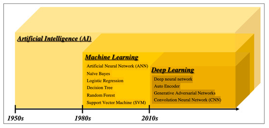
Figure 1. Overview of the development of artificial intelligence.
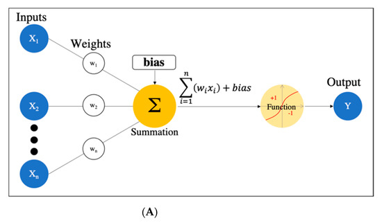
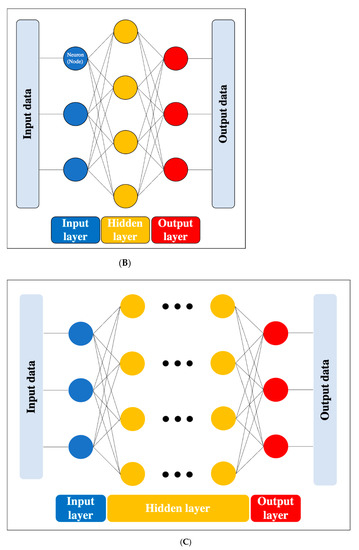
Figure 2. Artificial neural network. (A) Simple perceptron. (B) Neural network. (C) Deep neural network (DNN). Black dots: multiple hidden layers.
DL is a technology that utilizes a deep neural network (DNN), which is an ANN with four or more layers obtained by increasing the number of hidden layers. This enables handling problems that are not linearly separable and cannot be solved by the simple perceptron, as well as complex tasks and large amounts of data. (Figure 2c). However, we should be aware of issues such as overfitting and the vanishing gradient problem, which can occur as the DNN becomes deeper. Overfitting is a general phenomenon in ML where the model fits too well to the training samples, resulting in a low accuracy rate when evaluating unknown samples; in other words, the model is optimized for training data only and has no generality. To prevent overfitting, various efforts have been made to increase the amount of training data and regularize and simplify the models in ML model creation. The vanishing gradient problem is a phenomenon of multi-layered ANNs, in which the gradient approaches zero as it nears the input layer and finally disappears, resulting in a loss of learning. One way to solve this problem is to use the rectified linear unit (ReLU) instead of the sigmoid function for the activation function, which has been used in many DL studies. The ReLU function output is 0 if the input is a negative value, and the output is x if the input x is a positive value, such that the slope is 1, thus avoiding the vanishing gradient problem.
In conjunction with the significant advances in computer technology, such as graphics processing units (GPUs) with high computational power, the acquisition of large amounts of data through the development of the internet, and the development of various DL algorithms, including convolutional neural networks (CNNs) [18], autoencoders [19], and generative adversarial networks [20], have flourished, and various algorithms have emerged to further improve accuracy, solve enormous computational problems, and increase flexibility in learning. In particular, CNNs have been confirmed to be far superior to conventional image recognition methods and are now commonly used in medical imaging as well [21]; additional details about CNNs are described in 2.4 below.
2.2. Computer-Aided Diagnosis
Diagnosis based on image processing by computers is referred to as computer-aided diagnosis (CAD); the use of DL has become a mainstream AI application [22]. There are various roles in diagnostic imaging using computer systems, primarily computer-assisted detection (CADe) for lesion detection within an image, computer-assisted diagnosis (CADx) for differentiation (classification) of lesions, and segmentation for extraction of the area, including the contour of the object, which facilitates identifying the detailed delineation of the lesion and the category (i.e., lesion or organ) to which individual pixels belong. The basic technologies involved in the CAD schemes are (i) image processing such as normalization, (ii) image input, (iii) feature extraction, and (iv) results for detection or classification. In conventional CAD, each step of the process is conducted by human researchers themselves or with the help of computers, while DL-based CAD can automate this sequence of steps, end to end, through a learning process [23]. There are first reader, second reader, and concurrent reader forms of computer support, whereas the second reader type is the one most commonly found in CAD today. This is diagnosed first by the doctor, as usual; then, the computer results are reviewed, providing the possibility to change the interpretation and diagnose as necessary. On the other hand, a concurrent reader-type CAD system that refers to the CAD output at the same time as the diagnosis and a CAD system similar to the first reader type that makes a decision before the specialist’s diagnosis have also been developed [5].
2.3. Support Vector Machine
SVM is one of the supervised learning ML algorithms [16] (Figure 3). The basic concept is to classify data belonging to two categories by creating a boundary. When there are two types of data for classification, the boundary is a line; when there are three types, the boundary is a plane; and when there are four or more types, the boundary is a hyperplane boundary, which is collectively referred to as a “separating hyperplane”. A support vector represents the data closest to the separating hyperplane, and the distance between the support vector and the separating hyperplane is referred to as a margin; an SVM achieves classification by calculating the separating hyperplane such that this margin is maximized. (Figure 3a). If the data are linearly separable, this can be accomplished by a very simple calculation; however, in practice, including in imaging, data are generally not linearly separable. In such cases, soft-margin SVM and the kernel method are used to deal with the data. Essentially, soft-margin SVM allows a few anomalous expression profiles to fall on the “wrong side” of the separating hyperplane. Hence, introducing the soft margin necessitates introducing a user-specified parameter that roughly controls how far across the boundary data are allowed to be. There is a trade-off between hyperplane violations and margin distance, therefore ML classification is accomplished by trying to maximize the margin while allowing hyperplane violations as much as possible (Figure 3b). On the other hand, the concept of the kernel method is to map features to a high-dimensional feature space that is linearly separable (Figure 3c). However, this requires a huge amount of computation because features must be mapped to a number of dimensions as large as the number of data, so replacing the inner product of the non-linear map with a kernel function reduces the computational complexity significantly. This technique is called the kernel trick [24], for which several kernel functions can be used, such as Gaussian kernels, polynomial kernels, and radial basis function kernels. There are four main advantages of SVM: (i) the kernel trick allows application to nonlinear problems, (ii) the solution is theoretically unique due to the explicit criterion of margin maximization, (iii) generalizability is high due to margin maximization, and (iv) fewer parameters must be set in advance compared with neural networks. Nevertheless, SVM has several key disadvantages: (i) the effective features for classification must be determined manually, (ii) the learning time is huge when the number of data is large, (iii) some ingenuity is required to perform multi-class classification because it is basically a two-class classification method, and (iv) the output data do not give the probability of belonging to a classification category.
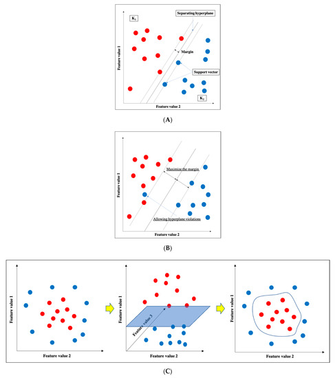
Figure 3. Support vector machine (SVM). (A) Basic structure of SVM. (B) Soft-margin SVM. (C) Kernel method.
2.4. Convolutional Neural Network
A CNN is a DL algorithm that was developed based on the processing of human visual signals (specifically, simulations of the principles of the cortical visual cortex V1 surrounding the avian sulcus in the occipital lobe). CNNs have made significant contributions to computer vision (the process by which a computer obtains and recognizes information from a series of images or videos) and continue to play a pivotal role in medical imaging analysis. In contrast to the feature extraction algorithms used in traditional CAD, which require human trial and error, CNNs use the image itself as an input and automatically learn to identify the most suitable features. In addition, conventional ANN has the problems of overfitting and vanishing gradient as the number of hidden layers increases; however, with CNNs, the layers are not fully connected, and the weights are adjusted for multiple data because multiple pixels in the input image (input feature map) share a single weight, thus preventing overfitting. The typical CNN consists of the following: (i) a convolutional and pooling layer for extracting distinctive features, and (ii) a fully connected layer for the overall classification. The input images are filtered by a number of specific filters automatically to extract the distinctive features to create multiple feature maps (Figure 4a). This operation for filtering is called convolution, and the process of training the convolutional filters to create the best feature maps is essential for success with CNNs. These feature maps are compressed to a smaller size in the pooling layer, and these convolution and pooling layers are repeated many times. Finally, a fully connected layer combines all the features to obtain the final result (Figure 4b). ReLU (used as an activation function to avoid the vanishing gradient problem) and data augmentation (used to increase the number of training images by performing micro-geometric transformations such as image inversion, resizing, and shifting) are commonly used to improve the generalizability of CNNs. In addition, the dropout technique is often used to prevent overfitting by randomly disabling some units in a layer and performing backpropagation in the remaining units [25]. Various CNN architectures, such as LeNet [26], Alexnet [27], GoogLeNet [28], VGGNet [29], and ResNet [30] have been proposed, and applications of them have been used in many kinds of research.
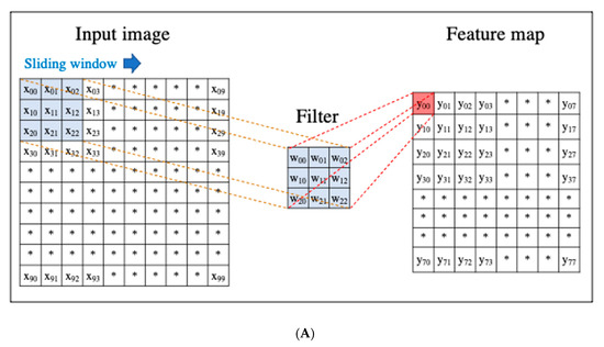
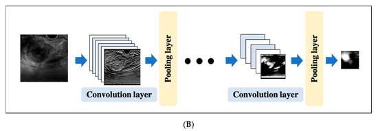
Figure 4. An example convolutional neural network (CNN). (A) Translation of an input image into a feature map in a convolution layer. (B) Layout of a deep convolutional neural network.
2.5. Validating Methods in Machine Learning
An important aspect of ML, including DL, is that the model learns the data such that it can accurately make predictions and classifications using unknown data. In other words, the model needs to acquire generalization performance. For this purpose, in the development of ML, the generalization performance of the model is necessarily validated, and there are several ways to achieve this, including the following approaches.
2.5.1. Hold out Validation
Some cases are randomly selected from the initial samples to form test cases, while the remaining cases are used for training. In general, it is often one-half, one-quarter, or one-nineth of the initial samples that are used for test cases. However, this is not suitable for the validation of a study with small amounts of data because of data bias.
2.5.2. K-Fold Cross-Validation
In K-fold cross-validation, the samples are divided into K groups, one of which is used as a test, and the remaining K-1 group is used for training. In cross-validation, each of the K groups of samples is tested k times, and the average of the tests is the cross-validation result. Although this method, depending on the number of patterns, is more computationally intensive than hold-out validation, it is currently widely used owing to its confidence and efficiency.
2.5.3. Leave-One-Out Cross-Validation
Only one sample is extracted from each of the N samples and used as test data, and the model is trained on the remaining N-1 samples and verified N times. More training data can be obtained than in the above two methods, but because the amount of computation is enormous in proportion to the number of samples, it is limited to studies with a relatively small number of samples.
References
- McGuigan, A.; Kelly, P.; Turkington, R.C.; Jones, C.; Coleman, H.G.; McCain, R.S. Pancreatic cancer: A review of clinical diagnosis, epidemiology, treatment and outcomes. World J. Gastroenterol. 2018, 24, 4846–4861.
- Egawa, S.; Toma, H.; Ohigashi, H.; Okusaka, T.; Nakao, A.; Hatori, T.; Maguchi, H.; Yanagisawa, A.; Tanaka, M. Japan Pancreatic Cancer Registry; 30th year anniversary: Japan Pancreas Society. Pancreas 2012, 41, 985–992.
- Kitano, M.; Yoshida, T.; Itonaga, M.; Tamura, T.; Hatamaru, K.; Yamashita, Y. Impact of endoscopic ultrasonography on diagnosis of pancreatic cancer. J. Gastroenterol. 2019, 54, 19–32.
- Van Dam, J.; Brady, P.G.; Freeman, M.; Gress, F.; Gross, G.W.; Hassall, E.; Hawes, R.; Jacobsen, N.A.; Liddle, R.A.; Ligresti, R.J.; et al. Guidelines for training in electronic ultrasound: Guidelines for clinical application. From the ASGE. American Society for Gastrointestinal Endoscopy. Gastrointest Endosc. 1999, 49, 829–833.
- Jiang, Y.; Inciardi, M.F.; Edwards, A.V.; Papaioannou, J. Interpretation Time Using a Concurrent‒Read Computer‒Aided Detection System for Automated Breast Ultrasound in Breast Cancer Screening of Women With Dense Breast Tissue. Am. J. Roentgenol. 2018, 211, 452–461.
- Abràmoff, M.D.; Lavin, P.T.; Birch, M.; Shah, N.; Folk, J.C. Pivotal trial of an autonomous AI‒based diagnostic system for detection of diabetic retinopathy in primary care offices. Digit. Med. 2018, 39, 20.
- Mori, Y.; Kudo, S.-E.; Misawa, M.; Saito, Y.; Ikematsu, H.; Hotta, K.; Ohtsuka, K.; Urushibara, F.; Kataoka, S.; Ogawa, Y. Real-Time Use of Artificial Intelligence in Identification of Diminutive Polyps During Colonoscopy: A Prospective Study. Ann Intern. Med. 2018, 169, 357–366.
- Goyal, H.; Mann, R.; Gandhi, Z.; Perisetti, A.; Ali, A.; Aman Ali, K.; Sharma, N.; Saligram, S.; Tharian, B.; Inamdar, S. Scope of Artificial Intelligence in Screening and Diagnosis of Colorectal Cancer. J. Clin. Med. 2020, 9, 3313.
- Kanesaka, T.; Lee, T.-C.; Uedo, N.; Lin, K.-P.; Chen, H.-Z.; Lee, J.-Y.; Wang, H.-P.; Chang, H.T. Computer-aided diagnosis for identifying and delineating early gastric cancers in magnifying narrow-band imaging. Gastrointest. Endosc. 2018, 87, 1339–1344.
- Lee, B.-I.; Matsuda, T. Estimation of Invasion Depth: The First Key to Successful Colorectal ESD. Clin. Endosc. 2019, 52, 100–106.
- Rosenblatt, F. The perceptron: A probabilistic model for information storage and organization in the brain. Psychol. Rev. 2006, 65, 386.
- Peng, F.; Schuurmans, D.; Wang, S. Augmenting naive bayes classifiers with statistical language models. Inf. Retr. 2004, 7, 317–345.
- Walker, S.H.; Duncan, D.B. Estimation of the probability of an event as a function of several independent variables. Biometrika 1967, 54, 167–179.
- Quinlan, J. Ross. Simplifying decision trees. Int. J. Man-Mach. Stud. 1987, 27, 221–234.
- Breiman, L. Random Forests. Mach. Learn. 2001, 45, 5–32.
- Vapnik, V. Statistical Learning Theory; Wiley: New York, NY, USA, 1998; Volume 1, p. 624.
- Rumelhart, D.E.; Hinton, G.E.; Williams, R.J. Learning representations by back-propagating errors. Nature 1986, 323, 533–536.
- LeCun, Y.; Bengio, Y.; Hinton, G. Deep learning. Nature 2015, 521, 436–444.
- Hinton, G.E.; Salakhutdinov, R.R. Reducing the Dimensionality of Data with Neural Networks. Science 2006, 313, 504–507.
- Salimans, T.; Goodfellow, I.; Zaremba, W.; Cheung, V.; Radford, A.; Chen, X. Improved Techniques for Training GANs. arXiv 2016, arXiv:1606.03498.
- Kido, S.; Hirano, Y.; Hashimoto, N. Computer-aided classification of pulmonary diseases: Feature extraction based method versus non-feature extraction based method. In Proceedings of the IWAIT2017; Institute of Electrical and Electronics Engineers (IEEE): Penang, Malaysia, 2017; pp. 1–3.
- Doi, K. Computer-aided diagnosis in medical imaging: Historical review, current status and future potential. Comput. Med. Imaging Graph. 2007, 31, 198–21111.
- Wu, D.; Kim, K.; Dong, B.; El Fakhri, G.; Li, Q. End‒to‒End Lung Nodule Detection in Computed Tomography. In International Workshop on Machine Learning in Medical Imaging; Springer: Cham, Switzerland, 2018; pp. 37–45.
- Noble, W.S. What is a support vector machine? Nat. Biotechnol. 2006, 24, 1565–1567.
- Yasaka, K.; Akai, H.; Kunimatsu, A.; Kiryu, S.; Abe, O. Deep learning with convolutional neural network in radiology. Jpn. J. Radiol. 2018, 36, 257–272.
- Lecun, Y.; Bottou, L.; Bengio, Y.; Haffner, P. Gradient-based learning applied to document recognition. Proc. IEEE 1998, 86, 2278–2324.
- Krizhevsky, A.; Sutskever, I.; Hinton, G.E. ImageNet Classification with Deep Convolutional Neural Net Works. Commun. ACM 2017, 60, 84–90.
- Szegedy, C.; Liu, W.; Jia, Y.; Sermanet, P.; Reed, S.; Anguelov, D.; Erhan, D.; Vanhoucke, V.; Rabinovich, A. Going deeper with convolutions. In Proceedings of the 2015 IEEE Conference on Computer Vision and Pattern Recognition, Boston, MA, USA, 7–12 June 2015; pp. 1–9.
- Simonyan, K.; Zisserman, A. Very Deep Convolutional Networks for Large-Scale Image Recognition. arXiv Preprint 2014, arXiv:1409.1556.
- He, K.; Zhang, X.; REN, S.; Sun, J. Deep Residual Learning for Image Recognition. In Proceedings of the 2016 IEEE Conference on Computer Vision and Pattern Recognition, Las Vegas, NV, USA, 26 June–1 July 2016; pp. 770–778.