+1 credit
| Version | Summary | Created by | Modification | Content Size | Created at | Operation |
|---|---|---|---|---|---|---|
| 1 | Angel Vázquez-Patiño | + 2513 word(s) | 2513 | 2020-08-23 07:54:53 | | | |
| 2 | Rita Xu | -1126 word(s) | 1387 | 2020-09-03 04:37:35 | | |
Video Upload Options
Physical processes govern climate at different spatial and temporal scales. These physical processes themselves constitute the transfer or flow of energy and mass. Causality methods have been used in recent years to study the flow of energy and mass. These methods give an indication of the direction of the flow and the intensity of the transfer. Climatic causal flows refer to hypotheses about physical processes that have been discovered using causal inference methods.
1. Introduction
Among the main components of the global water cycle and the atmospheric circulation are evaporation, circulation wind, and precipitation [1], and depicting their interplay is crucial to understand the dynamics of water vapor transport and the redistribution of energy. From a methodological perspective, most of the past studies that traced the pathways of humidity have used either numerical water vapor tracers, both in the Lagrangian approach (e.g., [1][2][3][4]) and the Eulerian approach (e.g., [5][6]), or physical water vapor tracers like the ones based on isotopes (e.g., [2][7]). Moreover, Drumond et al. [8] used Lagrangian and Eulerian approaches to complement each other. Meanwhile, Esquivel-Hernández et al. [2] and Windhorst et al. [7] complemented their isotope-based studies with Lagrangian water vapor tracers.
Recently, however, the use of complex networks to identify causal flows, indicative of matter and energy flows, has gained much ground in climatology. This is a data-based approach that has been explored to characterize flows [9] based on data only. This characterization is beneficial in two main ways [10]: (1) it provides more information on known physical processes and mechanisms, and (2) it allows one to hypothesize on those that were previously unknown. Very importantly, if methods such as complex networks (based solely on data) are not used, some new hypotheses or mechanisms cannot be possibly found since traditional methods generally impose assumptions based on prior expert knowledge. Thereby, complex networks could be exploited to expand understanding of the humidity and wind relationship with rainfall. When using causal networks, regions or in situ observations are represented by nodes in a network structure. The association between nodes can, in turn, represent different types of physically meaningful connections (e.g., [11][12]), for example, between humidity and rainfall. Often a scalar-valued field of some physical variable is used as a proxy to characterize the underlying vector field causing the dynamical processes (e.g., [10][13]). Some studies have used this approach to study rainfall over South America (e.g., [14][15]). Nevertheless, to the best of our knowledge, studies based on causal networks (a kind of complex network) to gain insights on humidity sources and pathways, or to unveil homogeneous zones of humidity and wind influence, do not yet exist.
Here, a virtual control volume approach that resembles the Eulerian description of a flow field but purely data-based in design is proposed, which uses a causal network approach to infer causal flows that allow the tracing of pathways of influence between climatic variables. To assess the proposed methodology, the rainfall from Ecuador is taken as a case study. Thus, it is possible to verify if the proposed approach reproduces known patterns of the influence that humidity and wind at different altitudes have on rainfall and to evaluate the ability of this approach to infer new ones. Continuous areas of influence are discussed based on the use of satellite-based rainfall observations and humidity and wind data from a reanalysis climate model.
The objective of this paper is to propose a causal discovery-based virtual control volume approach to study climate. With the approach, the aim is to provide new information on known relationships between humidity/wind and rainfall, but more importantly, identify new hypotheses regarding the direction and altitude of the influence of those critical variables.
2. Virtual Control Volume Approach to the Study of Causal Flows
The approach uses a virtual monitoring region (the virtual control volume), reminiscent of a control volume through which a continuum flows, as well as the control surface that encloses it. In our proposed methodology, outlined in Figure 1, a geographic region of interest (GRI) is enclosed by what has been named a virtual control surface where the flow of a physical quantity is analyzed (thick, larger, and straight arrows in Figure 1). This flow is indirectly detected, employing a causal inference method providing the direction of influence and its intensity. More concretely, the virtual control surface is made up of a finite arrangement of points (or pixels for raster data), which contain information on some climatic variables (e.g., humidity as in Figure 1a). In addition, in the enclosed geographic area, there is information on other climatic variables (e.g., rainfall as in Figre1b). Then, the influence from outside the virtual control volume is inferred using the information at the points on the corresponding virtual control surface as a proxy. In Figure 1, this influence is schematized with the curved arrows between the virtual control surface and the GRI, and the intensity with the thickness of the arrows.
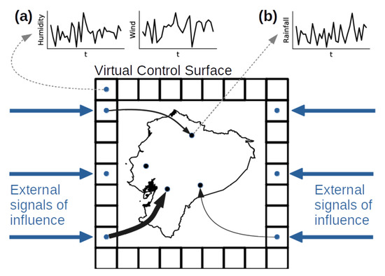
Figure 1. Outline of the proposed virtual control volume approach to study causal flows. The larger, straight arrows indicate the possible external influence towards the geographic region of interest (GRI). The control surface around the GRI is represented by the collection of squares, which contain time series of climatic variables that serve to infer external influence, e.g., humidity and wind (a). The causal flow is derived by employing a causality test between the climatic variable in the control surface (a) and a climatic variable in the GRI, e.g., rainfall (b). Arrows between the control surface and GRI indicate the existence of causal influence, and the thickness of the arrow indicates the intensity of the influence.
The continuous straight arrows in Figure 1 schematize the possible input signals that are characterized by the information that is available on the virtual control surface. Different processes act on different time scales from days to decades [16]. Thus, the time scale of the time series depicted in Figure 1a,b should be chosen according to the time scale at the processes of interest probably act.
In the case of the analysis of the influence of humidity and wind outside the GRI on the rainfall inside that region, the control surface is operationally defined as a set of specific points storing time series of humidity and wind. Besides, in the GRI (the control volume), there are rainfall time series either in specific positions or symmetrically arranged positions, e.g., from satellite observations or climate models. Inference from external influence can be carried out using a causal inference method such as Granger causality, which has been used to infer matter and energy flows in the climate system [11][12], or any others such as those based on the theory of information [17].
3. Study Area
Ecuador is located in the northwestern part of South America and is crossed by the equator as shown in Figure 2a. The presence of the Andean mountain range defines three climatic regions [18] whose limits are approximately at 1000 m a.s.l. both sides of the cordillera [19][20][21][22], i.e., the coast, Andean, and Amazon regions. Figure 2a shows the common spatial delimitation of the Andean region as the zones above the 1000 m a.s.l., the delimitation of the coast, west of the Andes, and the Amazon region, east of the Andes. The rainfall climatology is different in each region (Figure 2b), the Andes being the region with more heterogeneous spatiotemporal rainfall distribution due to the intricate western and eastern influences [23]. A unimodal rainfall distribution characterizes the coastal region with a peak from February to April. The Andean region has a bimodal distribution with peaks in February–March–April and October–November–December. Meanwhile, the distribution in the Amazon, although the more copious precipitation in the whole country, does not show high variability [21][24][25] but a peak exists from May to July. On the other hand, the spatial distribution of rainfall is heterogeneous in each region and with significant differences between the austral summer (DJF) and winter (JJA), as displayed in Figure 3.
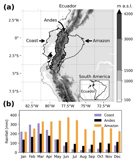
Figure 2. (a) Location, topography, and climatic regions of Ecuador as well as the resolution of NCEP/NCAR reanalysis data pixels used in the study (dashed lines); (b) mean rainfall by region based on data of Climate Hazards Group Infrared Precipitation with Stations (CHIRPS) (1981–2016).
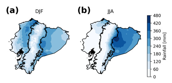
Figure 3. Monthly mean rainfall in (a) the austral summer (DJF) and (b) winter (JJA) from 1981 to 2016, based on CHIRPS data.
References
- Durán-Quesada, A.M.; Reboita, M.; Gimeno, L. Precipitation in tropical America and the associated sources of moisture: A short review. Hydrol. Sci. J. 2012, 57, 612–624, doi:10.1080/02626667.2012.673723.
- Esquivel-Hernández, G.; Mosquera, G.M.; Sánchez-Murillo, R.; Quesada-Román, A.; Birkel, C.; Crespo, P.; Célleri, R.; Windhorst, D.; Breuer, L.; Boll, J. Moisture transport and seasonal variations in the stable isotopic composition of rainfall in CENTRAL AMERICAN and ANDEAN PÁRAMO during EL NIÑO conditions (2015–2016). Hydrol. Process. 2019, 33, 1802–1817 doi:10.1002/hyp.13438.
- Sakamoto, M.S.; Ambrizzi, T.; Poveda, G. Moisture Sources and Life Cycle of Convective Systems over Western Colombia. Adv. Meteorol. 2011, 2011, 890759, doi:10.1155/2011/890759.
- Trachte, K. Atmospheric Moisture Pathways to the Highlands of the Tropical Andes: Analyzing the Effects of Spectral Nudging on Different Driving Fields for Regional Climate Modeling. Atmosphere 2018, 9, 456, doi:10.3390/atmos9110456.
- Arraut, J.M.; Satyamurty, P. Precipitation and Water Vapor Transport in the Southern Hemisphere with Emphasis on the South American Region. J. Appl. Meteorol. Clim. 2009, 48, 1902–1912, doi:10.1175/2009JAMC2030.1.
- Poveda, G.; Jaramillo, L.; Vallejo, L.F. Seasonal precipitation patterns along pathways of South American low-level jets and aerial rivers. Water Resour. Res. 2014, 50, 98–118, doi:10.1002/2013WR014087.
- Windhorst, D.; Waltz, T.; Timbe, E.; Frede, H.-G.; Breuer, L. Impact of elevation and weather patterns on the isotopic composition of precipitation in a tropical montane rainforest. Hydrol. Earth Syst. Sci. 2013, 17, 409–419, doi:10.5194/hess-17-409-2013.
- Drumond, A.; Marengo, J.; Ambrizzi, T.; Nieto, R.; Moreira, L.; Gimeno, L. The role of the Amazon Basin moisture in the atmospheric branch of the hydrological cycle: A Lagrangian analysis. Hydrol. Earth Syst. Sci. 2014, 18, 2577–2598, doi:10.5194/hess-18-2577-2014.
- Donner, R.V.; Lindner, M.; Tupikina, L.; Molkenthin, N. Characterizing Flows by Complex Network Methods. In A Mathematical Modeling Approach from Nonlinear Dynamics to Complex Systems; Macau, E.E.N., Ed.; Springer International Publishing: Cham, Switzerland, 2019; Volume 22, pp. 197–226, ISBN 978-3-319-78511-0.
- Ebert-Uphoff, I.; Deng, Y. Causal Discovery in the Geosciences—Using Synthetic Data to Learn How to Interpret Results. Comput. Geosci. 2017, 99, 50–60, doi:10.1016/j.cageo.2016.10.008.
- Hlinka, J.; Jajcay, N.; Hartman, D.; Paluš, M. Smooth information flow in temperature climate network reflects mass transport. Chaos Interdiscip. J. Nonlinear Sci. 2017, 27, 035811, doi:10.1063/1.4978028.
- Vázquez-Patiño, A.; Campozano, L.; Mendoza, D.; Samaniego, E. A causal flow approach for the evaluation of global climate models. Int J. Clim. 2020, 40, 4497–4517, doi:10.1002/joc.6470.
- Molkenthin, N.; Rehfeld, K.; Marwan, N.; Kurths, J. Networks from Flows-From Dynamics to Topology. Sci. Rep. 2014, 4, 4119–4123, doi:10.1038/srep04119.
- Ciemer, C.; Boers, N.; Barbosa, H.M.J.; Kurths, J.; Rammig, A. Temporal evolution of the spatial covariability of rainfall in South America. Clim. Dyn. 2017, 51, 371–382, doi:10.1007/s00382-017-3929-x.
- Guo, H.; Ramos, A.M.T.; Macau, E.E.N.; Zou, Y.; Guan, S. Constructing regional climate networks in the Amazonia during recent drought events. PLoS ONE 2017, 12, e0186145, doi:10.1371/journal.pone.0186145.
- Williams, P.D.; Alexander, M.J.; Barnes, E.A.; Butler, A.H.; Davies, H.C.; Garfinkel, C.I.; Kushnir, Y.; Lane, T.P.; Lundquist, J.K.; Martius, O.; et al. A Census of Atmospheric Variability From Seconds to Decades. Geophys. Res. Lett. 2017, 44, 11–201, doi:10.1002/2017GL075483.
- Runge, J.; Bathiany, S.; Bollt, E.; Camps-Valls, G.; Coumou, D.; Deyle, E.; Glymour, C.; Kretschmer, M.; Mahecha, M.D.; Muñoz-Marí, J.; et al. Inferring causation from time series in Earth system sciences. Nat. Commun 2019, 10, 2553, doi:10.1038/s41467-019-10105-3.
- Pourrut, P. (Ed.) El Agua en el Ecuador: Clima, Precipitaciones, Escorrentía; Estudios de Geografía; ORSTOM, Colegio de Geógrafos del Ecuador and Corporación Editora Nacional: Quito, Ecuador, 1995; Volume 7.
- Ulloa, J.; Ballari, D.; Campozano, L.; Samaniego, E. Two-Step Downscaling of Trmm 3b43 V7 Precipitation in Contrasting Climatic Regions With Sparse Monitoring: The Case of Ecuador in Tropical South America. Remote Sens. 2017, 9, 758, doi:10.3390/rs9070758.
- Ávila, R.; Ballari, D. A Bayesian Network Approach to Identity Climate Teleconnections Within Homogeneous Precipitation Regions in Ecuador. In Information and Communication Technologies of Ecuador (TIC.EC); Fosenca C, E., Rodríguez Morales, G., Orellana Cordero, M., Botto-Tobar, M., Crespo Martínez, E., Patiño León, A., Eds.; Springer International Publishing: Cham, Switzerland, 2020; Volume 1099, pp. 21–35, ISBN 978-3-030-35739-9.
- Ballari, D.; Giraldo, R.; Campozano, L.; Samaniego, E. Spatial functional data analysis for regionalizing precipitation seasonality and intensity in a sparsely monitored region: Unveiling the spatio-temporal dependencies of precipitation in Ecuador. Int J. Clim. 2018, 38, 3337–3354, doi:10.1002/joc.5504.
- Campozano, L.; Ballari, D.; Celleri, R. Imágenes TRMM para identificar patrones de precipitación e índices ENSO en Ecuador. Maskana 2014, 5, 185–191.
- Campozano, L.; Célleri, R.; Trachte, K.; Bendix, J.; Samaniego, E. Rainfall and Cloud Dynamics in the Andes: A Southern Ecuador Case Study. Adv. Meteorol. 2016, 2016, 3192765, doi:10.1155/2016/3192765.
- Morán-Tejeda, E.; Bazo, J.; López-Moreno, J.I.; Aguilar, E.; Azorín-Molina, C.; Sanchez-Lorenzo, A.; Martínez, R.; Nieto, J.J.; Mejía, R.; Martín-Hernández, N.; et al. Climate trends and variability in Ecuador (1966-2011). Int. J. Climatol. 2016, 36, 3839–3855, doi:10.1002/joc.4597.
- Tobar, V.; Wyseure, G. Seasonal rainfall patterns classification, relationship to ENSO and rainfall trends in Ecuador. Int. J. Climatol. 2018, 38, 1808–1819, doi:10.1002/joc.5297.