CFD Modelling of Slurry Flows

Version	Summary	Created by	Modification	Content Size	Created at	Operation
1		Oluwaseun Adedeji	+ 5435 word(s)	5435	2021-09-10 12:04:54	\|
2	The format is correct	Lindsay Dong	Meta information modification	5435	2021-09-14 04:55:13	\|

This entry is adapted from the peer-reviewed paper 10.3390/pr9091566

Slurry pipe transport has directed the efforts of researchers for decades, not only for the practical impact of this problem, but also for the challenges in understanding and modelling the complex phenomena involved. The increase in computer power and the diffusion of multipurpose codes based on Computational Fluid Dynamics (CFD) have opened up the opportunity to gather information on slurry pipe flows at the local level, in contrast with the traditional approaches of simplified theoretical modelling which are mainly based on a macroscopic description of the flow.

slurry pipe flows computational fluid dynamics Eulerian–Lagrangian model Eulerian–Eulerian model two-fluid model mixture model slurry erosion

1. Introduction

1.1. Engineering Aspects and Physical Features of Slurry Pipe Transport

Hydraulic transport of solid particles in the flow of carrying liquid is of great importance in many industries, including mining, dredging, oil and gas, chemistry, agriculture or waste treatment ^[1]^[2]^[3]^[4]^[5]. In those applications, it can pose a reliable, safe, economic and environmental-friendly alternative to other means of transportation as for instance trucks.

The broad variety of environments in which the solids hydrotransport is applied produces different solid–liquid mixtures to be pumped and conveyed primarily through pressurized pipes. Water is typically the carrying liquid but the carried solids can be very different from very fine to very coarse and from very heavy to very light. The two phases (liquid and solid) interact with each other while flowing in a conduit and significantly affect the behavior of the mixture flow. This paper discusses transport in pressurized pipes and focuses on turbulent flows of mixtures (slurries) composed of Newtonian carrier and particles coarse and/or heavy enough to alter the internal structure of the flow by causing an asymmetrical distribution of velocity and non-uniform distribution of solids in the cross section of a pipe. In such flows, called settling slurry flows, the solid particles interact with turbulent eddies of the flowing carrier and may also interact with each other through interparticle collisions or longer-lasting contacts ^[6]^[7]^[8].

Essentially, there are three basic types of settling slurry flow. At one extreme is the pseudo-homogeneous regime, typical of flows laden with fine particles (typically fine sand of particle sizes between 60 and 200 microns) flowing at high velocity. Their submerged weight is carried by fluid support mechanisms associated with flow turbulence. The distribution of suspended particles is close to uniform although some gradient usually occurs in the pipe cross section, see Figure 1a. Viscous friction is responsible for flow energy loss. The other limiting case is represented by the fully-stratified regime, typical of flow conveying large, rapidly-settling particles at low velocity. Their submerged weight cannot be carried by flow turbulence and they travel in the lower part of the pipe by saltation, or as a sliding bed (Figure 1c). Particle contacts with each other and with a pipe wall considerably contribute to the overall flow friction. The intermediate case, for which both inter-granular contact and fluid support mechanisms are significant, is called heterogeneous flow (Figure 1b). For relatively large particles, the heterogeneous flow regime can be more distinctly stratified with a detectable sliding bed and the transported grains can be supported either by turbulent eddies or by mutual collisions above the sliding bed. Additionally, often encountered in practice is the flow of broadly graded solids in a Newtonian carrier in which particles of quite different sizes and supported by different mechanisms interact with each other. Overall, the behavior of the discussed slurry flows is quite complex as it is a result of the number of different mechanisms governing the flow and being responsible for particle support and friction.

Figure 1. Different patterns of settling slurry flow in horizontal pipes (a) pseudo-homogeneous flow (b) heterogeneous flow (c) fully-stratified flow. The colors of the particles identified their basic transport mechanism, namely, interaction with the turbulent fluid (grey), quick collision with other particles (green), and long-lasting contacts with nearby particles (red).

Settling slurries tend to stratify in the pipeline and the degree of stratification affects both the pipeline resistance and transport safety. Typically, the pipeline resistance is quantified by the frictional pressure drop over the length of the pipe, whereas the transport safety is evaluated by the flow velocity, which must exceed the minimum safe velocity at which the system should operate without the danger of accumulation of particles in the form of a deposit at the bottom of the pipe which may result in pipe blockage. The operating velocity at which first grains stop moving and start to form the deposit is called the deposition-limit velocity and it is one of the key parameters in a description of slurry flow for purposes of design or operation of a slurry transport system typically composed of a pipeline and a pump ^[9]^[10].

1.2. Modeling of Slurry Pipe Flows

Predictive models are essential design tools for slurry transport systems. In this perspective, the prediction of the pipe characteristic curve is one of the key tasks of slurry flow modelling, and another major task is to predict the deposition-limit velocity, Vdl, which is the value of flow velocity below which solid deposit is observed. A more detailed prediction of slurry flow includes information on the internal structure of the flow in the form of distributions of local velocity and concentration (e.g., ^[11]) which helps to understand the friction and to predict other phenomena, such as the erosive wear of a pipe wall.

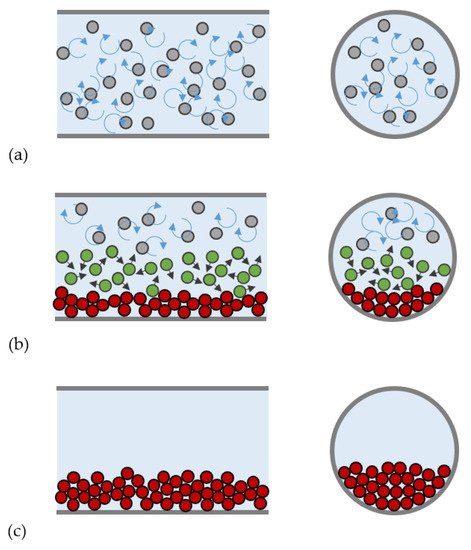
There are several sorts of models available for predictions of the slurry flow quantities. It has been shown that different slurries can form quite different flow types with different flow patterns and it must be emphasized that the different slurry flows exhibit rather different flow behaviors ^[12]^[13]. An identification of the flow type is essential for the successful modelling of slurry flows and prediction of their behavior in a pump-pipeline transport system. The available models rely on different approaches, which have different levels of complexity and refinement, so that, in principle, simpler approaches are easier to use but provide less refined outputs.

1.3. The Potential of Computational Fluid Dynamics

The complexity of solid–liquid flow as is the flow of settling slurry demands that the flow behavior is best analyzed on a local level by monitoring distributions of flow quantities throughout the flow domain. This requirement focuses attention on Computational Fluid Dynamics. Traditionally, CFD simulations for engineering purposes have been restricted to simpler one-phase flows primarily due to limitations in computer power and the capability of CFD codes. However, current advancements in this field have enabled to increase the amount of research work on the numerical simulation of pipe flows of slurry exponentially in few years, opening the way to the use of this approach for the engineering applications.

2. CFD Modelling Approaches

2.1. Eulerian–Lagrangian Modelling

In the Eulerian–Lagrangian (EL) approach, the carrier liquid is modelled as a continuum, and therefore normally referred to as the continuous phase in a multiphase flow simulation. For an isothermal flow, the mass and linear momentum equations must in general be solved:

where μeffl represents the effective viscosity of the liquid, and it is calculated as the sum of the molecular viscosity μl and the eddy viscosity μtl, and Pl is equal to the time-averaged pressure pl plus 2/3ρlkl. There are a number of models for computing the turbulence viscosity, such as k-?, SST k-ω, and Spalart–Allmaras. As it is not the purpose of this article to discuss these models, the reader is referred to Menter ^[14], Launder and Spalding ^[15] for further information and theoretical background. Equations (12) and (13) or (10), along with the turbulence model equations, form the basis for the Eulerian fashion as applied to the liquid.

Generally, the fluid flow equations discussed here above are numerically solved using grid-based methods such as the Finite Volume Method, the Finite Difference Method, or the Lattice–Boltzmann Method ^[16]. Depending on the ratio of mesh size to particle diameter, Eulerian–Lagrangian models can be classified into point-particle (or unresolved) methods and fully-resolved methods. If the particle dimensions are negligible as compared to the fluid cell, then the point-particle approximation can be made, which consists in assuming that the particles are point sources of momentum with zero dimension (Figure 2a). At the opposite extreme, fully-resolved methods require the grid size to be much smaller than the particle size and model accurately the flow around the solid particle (Figure 2b). Such point-particle approximation is generally made in Euler–Lagrange simulations for engineering purposes, although a fully-resolved treatment is feasible with supercomputing resources.

Figure 2. Main modelling approaches in the Eulerian–Lagrangian framework: (a) point-particle approach (b) fully-resolved approach.

In both approaches, the equation of motion for each particle is based on Newton’s second law. Each particle is tracked individually throughout the fluid domain. In particular, it is important to solve for the angular momentum in pipe flows, because collisions with walls are frequent. The trajectory, linear momentum and angular momentum conservation equations for a rigid, constant-mass particle can be written as:

The evaluation of the fluid–particle forces and torques is carried out differently in fully resolved and point-particle models. Since, in fully-resolved models, the mesh resolution is much smaller compared to the particle size, the action from the fluid to a particle can be directly obtained by integrating the pressure and viscous stresses distributions over the particle surface (Figure 6b). Conversely, in point-particle models, the forces and torques on the RHS of Equations (15) and (16) cannot be computed directly. Thus, correlations for the external forces and torques acting on each particle must be obtained from appropriate force models, devised either from experiments or from surface-resolved Direct Numerical Simulations.

Models for liquid-to-particles surface forces include, among others, drag, shear-induced lift, pressure gradient and virtual mass. The drag force is often the dominant one in liquid–solid flows, and it is calculated as:

As discussed, point-particle methods and fully-resolved methods impose strict constraints on the size of the grid used for fluid flow calculation, which must be much larger and much smaller compared to the particle diameter, respectively. In order to translate this concept into practical recommendations, threshold values must be given for the ratio of mesh size to particle diameter. It was reported ^[17] that, in fully-resolved methods, the mesh size should be at most 1/8 of the particle diameter so that numerical errors can be limited. Increasing the ratio of mesh size to particle diameter, e.g., bigger than 1/5, can lead to rough representation of particle boundary and thus inaccurate results. To avoid an undesirable increase in computing power when using a fine mesh throughout the whole computing area, it is possible to use the local dynamic mesh refinement close to the particle surface ^[17]. However, still, the fully-resolved method is suitable only for processes where the number of particles is limited (in the order of hundreds or thousands). As an example of the largest systems studied with this approach, in ^[18] simulations of river bed forms were carried out on 24,756 cores, and only 350,000 particles were tracked, which is much less than the point-particle methods, where the number of particles can reach tens of millions. At the opposite extreme, the literature showed that not only the basic idea underlining point-particle models, but also the accuracy of widely used force models are affected by the grid size. Peng et al. ^[19] recommended that, in order to ensure the accurate calculation of the relative velocity and the void fraction in different drag force models, the mesh size should be at least three times larger than the particle diameter. Otherwise, by reducing the ratio of mesh size to particle diameter to smaller than 3, the drag force model can be inaccurate with a large deviation from experimental results. Apparently, for the EL modelling of particulate flows, there exists a grey zone, as, if the ratio of mesh size to particle diameter ranges from 1/8 to 3, both point-particle and fully-resolved modelling are not accurate. There is a clear gap for the situations with a size ratio ranging from 1/8 to 3. In order to bridge it, several approaches have been proposed, such as the statistical kernel method, the porous cube method, the big sphere method and the diffusion approach ^[20].

2.1.1. One-Way Coupled Slurry Flows

Equations (12)–(16) form the basis of the Eulerian–Lagrangian approach. Particles are directly affected by the fluid flow, since the forces and torques are partly caused by the fluid. However, this set of equations, as they are herein presented, do not account for the effect of the particles on the fluid flow. This is the one-way coupling regime, is valid only in flows with a low particle concentration (Figure 3). Depending on the local particle concentration, the impact of the particles on the fluid cannot be disregarded. In such cases, the reaction of the particles to the fluid must be taken into account. Additionally, interparticle collisions may play a role. These will be dealt with in the following sections.

Figure 3. Classification of flow particle-laden flows according to the coupling regime and of the key physical mechanisms driving the flow. The distinction between disperse and dense flows has been proposed by Loth ^[21], whereas that between dilute and dense flows, including the limits to the solid volume fraction, is obtained from the map of Elghobashi ^[22].

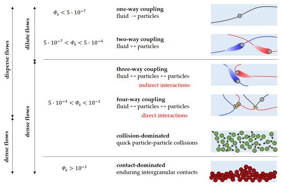
2.1.2. Two and Four-Way Coupled Slurry Flows

In the two-way coupling regime, and under the point-particle approximation, the momentum exchanged between the particle and the fluid must be added to the RHS of Equation (13):

where the summation applies to all parcels contained in volume W. In compliance with Newton’s Third Law, body forces should not be considered. In Equation (19), it is assumed that only body forces experienced by the particles are weight and buoyancy. Another peculiar feature of two-way coupled Eulerian–Lagrangian models resides in the presence, in the equations of the turbulence model, of source terms associated with the influence of the particles on the turbulence characteristics of the carrier fluid. This phenomenon is called turbulence modulation, and it is characteristic of the two-way coupling regime; particularly, the evidence shows that fine particles tend to attenuate the turbulence in the carrier fluid phase, whereas turbulence enhancement occurs in the case of coarse solids ^[22].

Particle-to-particle collisions may become important at higher concentrations. Even under “disperse” operating conditions, in the sense given by Loth ^[21] (Figure 3), interparticle collisions may be important in redispersing particles in pipe flows, acting as a diffusion mechanism, especially in locally concentrated regions. If they are to be considered, we then have the so-called four-way coupling. There are different possibilities for modelling such forces: hard-sphere and soft-sphere models exist. In the latter, the mechanical properties of the particle material must be used to calculate the tiny deformation that occurs during a collision, while the former assumes that particles are perfectly rigid. The Discrete Element Method (DEM) commonly employs a soft-sphere model, using one of the several models available for normal contact forces, namely linear spring–dashpot, and non-linear damped Hertzian spring–dashpot, among others. The soft sphere model requires determining the normal spring stiffness coefficient of the linear model through the numerical solution for the overlap between particles in non-linear models. Irrespective of the interparticle collision model, a coarse-graining procedure is needed in accordance with the parcel concept, except for very dilute systems for which every single particle can be represented.

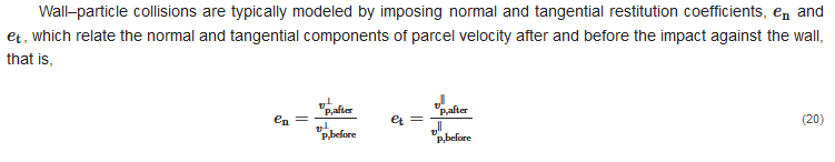
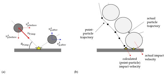
2.1.3. Boundary Conditions

Regarding boundary conditions for slurry flows in pipes, normally when the interest is in the fully developed flow, periodic conditions are applied to a pipe length (Figure 4a). A pressure drop or source term forcing a given mass flow must be prescribed as the driving force. Otherwise, classical inlet and outlet boundaries are used, i.e., the convective flux of the liquid, along with the turbulence quantities, are prescribed at the inlet boundary, whereas at the outlet the static pressure is specified and the normal gradient is zero for all liquid variables (Figure 4b). As for the particles, they are normally injected at the inlet with a given velocity, and are allowed to escape the outlet. It is worth noting that the applied boundary conditions scheme affects the length of pipe to be simulated to achieve fully developed flow. In fact, whereas a short pipe length is sufficient in the case of periodic boundary conditions, the domain must be longer if inlet–outlet conditions are used, since the flow must develop from the state imposed at the inlet boundary. Assessing the length of the pipe to be simulated is a significant feature of slurry pipe flow simulations.

Figure 4. Typical boundary condition schemes in the simulation of slurry pipe flows.

In both schemes, the pipe walls are treated as solid wall boundaries. No-slip conditions are adopted whenever the mesh resolution is enough to calculate the boundary layer profile. Alternatively, if not enough refinement is possible, the wall shear stress according to a given law-of-the-wall, such as Launder and Spalding’s ^[23], and different types of constraints on the turbulent variables are applied. As with other wall-bounded flows, the wall boundary conditions play an important role in pipe flows. This is because upon colliding with a wall, the particle exchanges linear and angular momentum. This may translate into an increase in the flow pressure drop, especially for horizontal flows, and more so for rough pipes. After a collision, the particle must be reaccelerated by the fluid. In order to maintain the mean fluid velocity, this reacceleration comes at the expense of increased inlet pressure. As demonstrated by Huber and Sommerfeld ^[24], wall roughness can play a very important role in horizontal pipe flows.

where all symbols are indicated in Figure 5a. An important feature that deserves some attention is that, although the derivation in ^[25] accounts for the particle finite radius during collisions, most implementations of the Euler–Lagrange approach are performed under the point-particle approximation and they estimate the collision as if occurring at the wall (Figure 5b).

Figure 5. (a) impact of a particle against a wall; (b) deviation between a trajectory calculate under the point-particle assumption and the actual particle trajectory in the proximity of a wall.

2.2. Eulerian–Eulerian Modelling (Two-Fluid Modelling)

2.2.1. Fundamental Conservation Equations

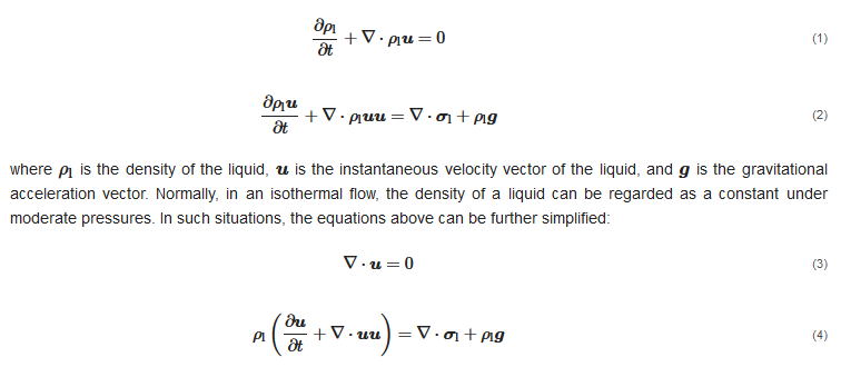
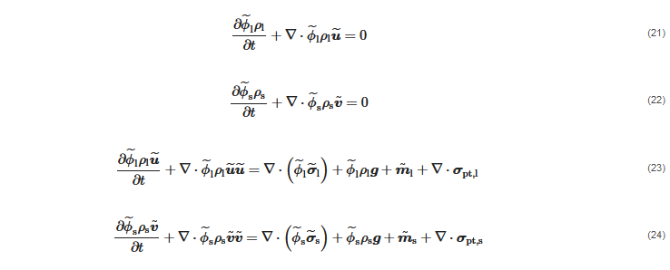
In the Eulerian–Eulerian approach, both phases are interpreted as interpenetrating continua and they are modelled in the Eulerian, cell-based framework. This is achieved by solving for the fundamental mass and momentum conservation equations for two media, namely, the carrier liquid and a fictitious fluid representing the fluid dynamic behavior of the ensemble of solid particles, called “solid phase”. The instantaneous equations of the two-fluid model can be derived in different ways, and they typically read as follows:

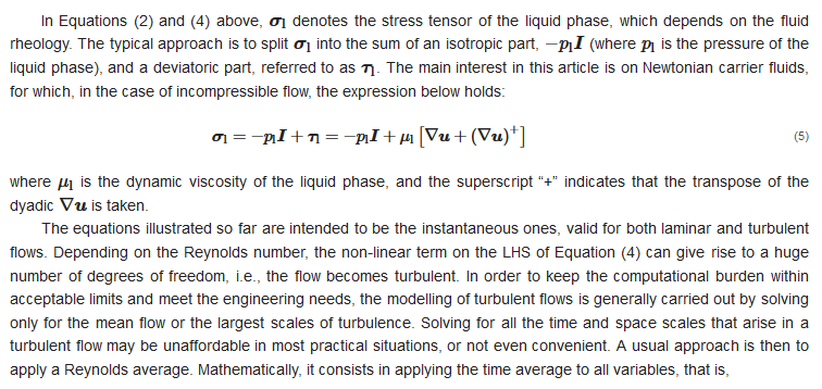
2.2.2. Constitutive Equations

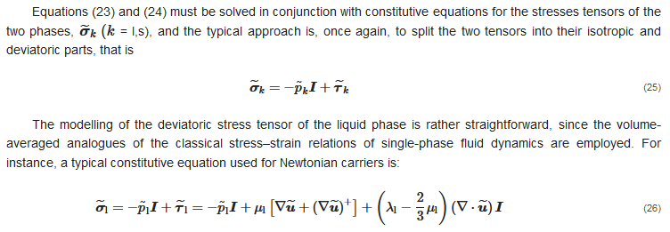
where λl is called the second viscosity coefficient. Note that, in principle, the volume-averaged velocity field u˜ is not divergence-free for incompressible carriers. Therefore, the last term in Equation (26) is not identically zero, even if it is usually neglected in Euler–Euler models, obtaining a formally similar relation as in the classical Eulerian–Lagrangian approach (Equation (5)). However, the situation becomes more complicated for the solid phase. Solving Equation (25), in fact, requires facing the non-trivial challenge of how to characterize from a physical point of view (first) and how to evaluate (afterwards) the pressure and deviatoric stress tensor of the solid phase. Generally, a solid-phase analogous of Equation (26) is employed, as follows:

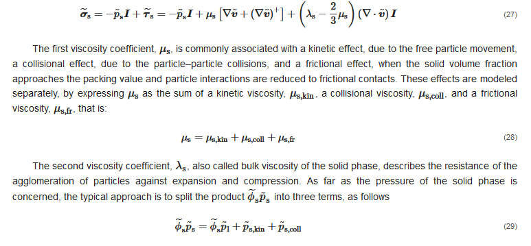
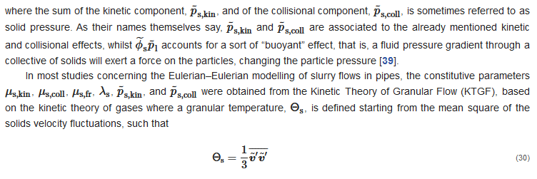
In the KTGF, the six variables listed above are algebraic functions of Θs as well as other particle-related parameters, such as the restitution coefficient of particle–particle collisions, the solid volume fraction at maximum packing, and the angle of internal friction. The granular temperature, in turn, is obtained from the solution of its own transport equation. However, other two-fluid models for slurry pipe flow simulation do not rely on the KTGF but use empirical constitutive equations for μs and p˜s. As far as μs is concerned, a possible approach was mentioned in [39], which consists in estimating μs from the viscosity of the mixture μm.

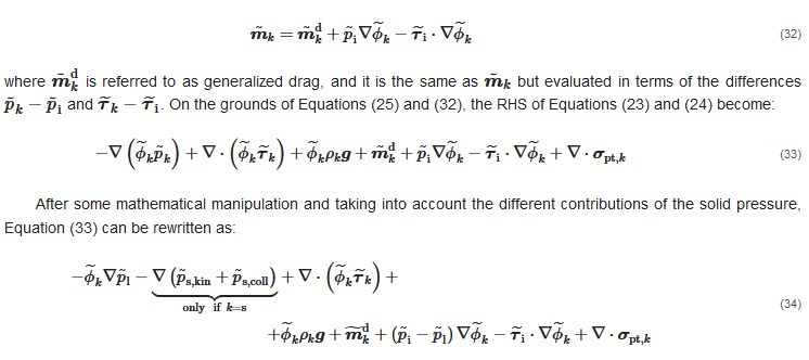
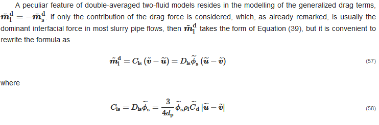
2.2.3. Interfacial Momentum Transfer

The terms m˜k (k = l,s), called interfacial momentum transfer terms, account for the exchange of forces between the two phases through their interface. Following Enwald et al. [39], these parameters can be expressed in terms of the interfacially-averaged pressure and deviatoric stress tensor, p˜i and τ˜i, as follows:

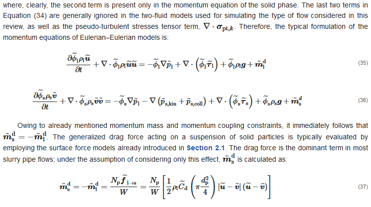
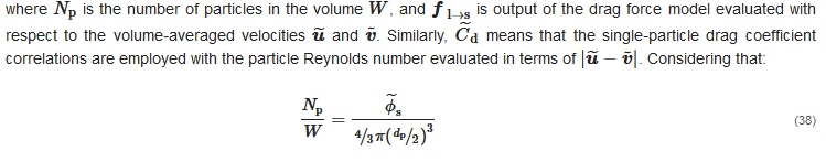
it is possible to rewrite Equation (37) as

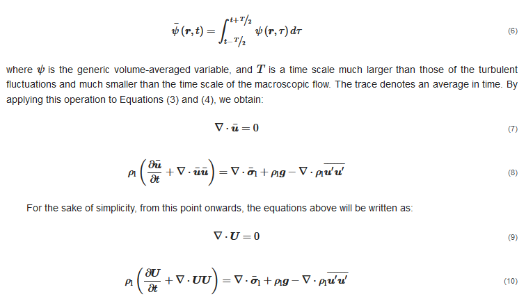
2.2.4. Modelling of Turbulent Flows

The equations illustrated so far are intended to be the instantaneous ones, valid for both laminar and turbulent flows. However, to keep the computational burden within acceptable limits and meet the engineering needs, the modelling of turbulent flows is generally carried out by solving only for the mean flow or the largest scales of turbulence. However, the Eulerian–Eulerian analogous of the RANS approach for single-phase flow is definitely complex to derive, as well as to characterize and justify from a physical point of view. In this regard, the double-average approach provides a strong mathematical ground for the derivation of the two-fluid models for turbulent flows. Essentially, the idea is to start from the instantaneous, volume-averaged equations and apply a second averaging operator, obtaining double-averaged equations whose unknowns are the double-average of the fluid dynamic variables (pressure, velocity, volume fraction, etc.). For the second averaging operator, two main options have been documented in the literature. The former consists of applying the same time average operator in Equation (6) to all volume-averaged variables, that is,

The latter option is to use the time average for all variables except for the velocity, to which the Favre operator is applied

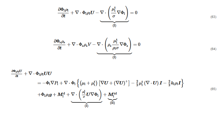
As illustrated by Burns et al. ^[26], the fundamental conservation equations assume different forms according to the second averaging operator applied. This is immediately evident in the mass conservation equations. After time-averaging, the mass conservation equations become:

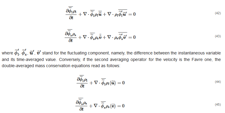
Comparing the two sets of equations above indicates that, when time-averaging of the volume-averaged mass conservation equations is performed, two additional terms come up, associated with the double correlations between the fluctuating velocity vector and the fluctuating volume fraction. These terms require modelling, which is typically achieved through the gradient diffusion approximation, initially proposed by Spalding ^[27] based on an analogy between the turbulent dispersion of solid particles and the turbulent diffusion of a passive scalar:

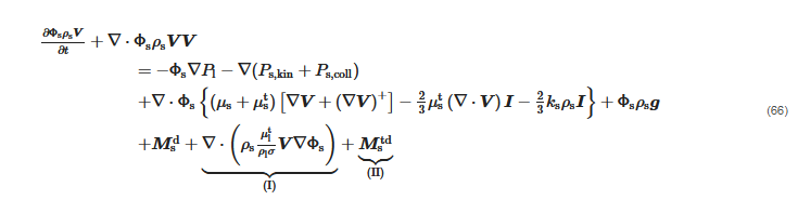
Whatever the second averaging operator is, double averaging of the momentum conservation equations produces several terms depending on double and triple correlations between fluctuations, which need to be modelled by additional closures. Elghobashi and Abou-Arab ^[28] reported the equations obtained by time-averaging the volume-averaged equations, and the momentum ones consist of about 15 terms. Most of these terms are simply ignored in commonly used two-fluid models, either because they are small or difficult to estimate. One might think that ignoring some terms might deviate the numerical solution from the physical one. However, it should be borne in mind that closure correlations are never exact, but they rely on approximations and empiricism: therefore, there is no guarantee that adding more closures results in higher accuracy, unless there is no doubt that such closures are applicable to the specific case study under investigation.

Given that, the double correlations associated with the convection terms are usually taken into account in slurry flow simulations. In the case of time-averaging of all variables, they are as follows:

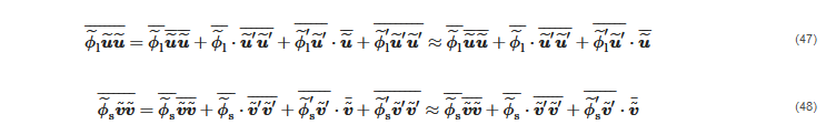
whilst, if the volume-average velocity is Favre-averaged, the form of the double-averaged convection terms is:

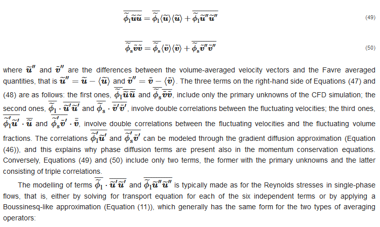
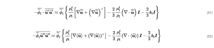
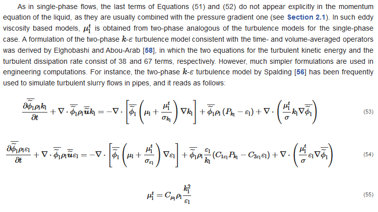
As in single-phase flows, the last terms of Equations (51) and (52) do not appear explicitly in the momentum equation of the liquid, as they are usually combined with the pressure gradient one (see Section 2.1). In such eddy viscosity based models, μtl is obtained from two-phase analogous of the turbulence models for the single-phase case. A formulation of the two-phase k-ε turbulence model consistent with the time- and volume-averaged operators was derived by Elghobashi and Abou-Arab [58], in which the two equations for the turbulent kinetic energy and the turbulent dissipation rate consist of 38 and 67 terms, respectively. However, much simpler formulations are used in engineering computations. For instance, the two-phase k-ε turbulence model by Spalding [56] has been frequently used to simulate turbulent slurry flows in pipes, and it reads as follows:

Mandø et al. ^[29] identified the main criticism of turbulence modulation models in the fact that, according to their derivation, they can predict only either turbulence attenuation or turbulence enhancement, as typical of particle-laden flows with fine and coarse particles, respectively. In order to overcome such limitations, these authors proposed a comprehensive model which can predict both effects at the same time. Such model, employed for simulating gas–solid flows using the Eulerian–Lagrangian approach, which was later generalized and applied to the Eulerian–Eulerian modelling of slurry flows in vertical pipes by Messa and Malavasi ^[30]. However, a key issue is that all available correlations were developed for dilute flows in the two-way coupling regime, for which the solid content is much lower compared to the high concentrations encountered in hydro-transport applications. The effect of turbulence modulation on the behavior of dense slurry flows, and its modelling, is an open problem. Indeed, in some papers the same expressions of the source term derived for dilute flows have been applied to dense liquid–solid flows in pipes, using the KTGF and empirical formulas for evaluating the correlations between the fluctuating velocities (e.g., ^[31]); however, no discussion was provided around the validity of such approach, nor it was assessed the actual impact of these terms on the CFD solution.

According to Burns et al. ^[26], a reasonable first approximation is to treat $D_{ls}$ as constant during the averaging process. Under this assumption, time-averaging of Equation (57) yields:

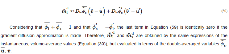
Conversely, if expressed in terms of the Favre-averaged velocities, Equation (59) becomes:

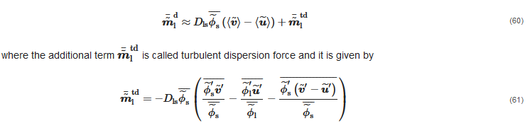
On the grounds of what was stated before, when introducing the gradient-diffusion approximation, the last term disappears, whilst the first two can be arranged, yielding:

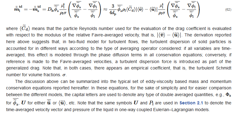
where the phase diffusion terms (I) and the turbulent dispersion force (II) are mutually exclusive of each other.

2.2.5. Boundary Conditions

Particularly, in the periodic scheme, the fluid dynamic characteristics of both phases are imposed to be the same at the first and last slabs of cells, and the total mass flow rates of the two phases are specified. Conversely, in the inlet–outlet scheme, which is the most commonly employed in the two-fluid framework, the conditions are as follows. The convective flux of each transported variable must be specified in all surface cells of the inlet boundary, and, practically speaking, this requires imposing the distributions of the locally averaged volume fractions and velocities of the two phases, in addition to those of the turbulent parameters, such as k and ε, and, in the case of KTGF-based models, also that of the granular temperature, Θs. At the outlet boundary, the pressure of the liquid phase is specified and held constant, and the normal gradient of all other variables are zero.

Whatever the boundary conditions scheme is, the pipe walls are treated as solid wall boundaries. The conditions imposed to the carrier fluid phase are very similar to those of single-phase flow simulations, that is, zero advection flux from all surface cells, the prescribed value of wall shear stress according to a given law-of-the-wall, such as Launder and Spalding’s ^[23], and different types of constraints on the turbulent variables. Conversely, the modelling of the wall boundary conditions for the solid phase is one of the key issues in the Eulerian–Eulerian modelling of slurry pipe flows, since this feature has a considerable impact on the prediction of the additional flow resistance owing to the presence of the particles. Sometimes, a no-slip condition is applied to the wall solid phase velocity, whereas a more commonly used option in two-fluid models based on the KTGF is the partial slip condition of Johnson and Jackson ^[32]. Messa and Malavasi ^[33] developed a solid wall boundary condition for application to slurry flows in pipeline systems, which is based on a blending between a log-law wall function for small particle sizes and an empirical, Bagnold-like formula for big particle sizes.

2.2.6. Multi-Fluid Modelling

An extension of the two-fluid model to an arbitrary number of dispersed phases is proposed, which is called a multi-fluid model. In the simulation of slurry pipe flows, the multi-fluid model could be employed for application to slurries with broadly graded particle size distribution. This is achieved by dividing the particles into

n_{d}

classes, each characterized by representative particle size, and solving for

n_{d}

pairs of mass and momentum conservation equations for the solid phase, in addition to the corresponding equations for the carrier liquid. Clearly, the

n_{d}

+1 phases are subjected to mass coupling, meaning that the volume fractions must sum up to a unit value, and to momentum coupling, through the action–reaction principle. Particularly challenging is the modelling of the momentum transfer among the phases, noting that these include both the interactions between the carrier liquid and each individual solid phase, through the fluid–particle forces, and those between two solid phases, generated by the collisions and contacts between particles of different sizes. Conversely, the collisions between particles belonging to the same size class are accounted for through the constitutive equations for the stresses tensor of that class. In the few applications of the multi-fluid model to slurry pipe flows reported in the literature, two particle classes are considered, and the closure and constitutive equations were obtained from the KTGF.

2.3. Mixture Modelling

The mixture model can be regarded as a simplified formulation of the multi-fluid model, which is applicable only under specific assumptions on the flow. Perhaps the most complete overview of the mixture model was provided by Manninen et al. ^[34], who derived the fundamental equations starting from the Eulerian, double-averaged mass and momentum conservation equations of each phase. For the sake of simplicity, the origin of the mixture model equations will be explained for a slurry with a narrow particle size distribution, for which a single dispersed phase can be defined. However, the main strength of the mixture model resides in the fact that it can be easily extended to an arbitrary number of dispersed phases; this is particularly useful, for instance, to simulate slurry flows with broadly graded particle size distribution without incurring into the high computational burden and numerical criticisms of multi-fluid models.

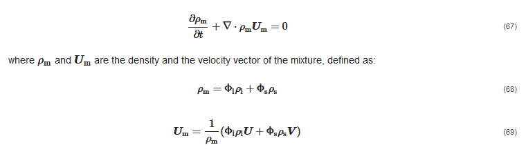
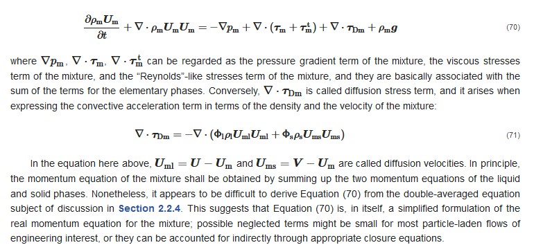
2.3.1. Fundamental Conservation Equations

As its name implies, the primary variables of the mixture model are the properties of the mixture, intended as the sum of the two phases. The mass conservation equation for the mixture is obtained by summing up the corresponding equations of the individual phases. If we assume that the double-averaged velocities are the Favre-averaged ones, so that no phase diffusion terms appear in the continuity equations, by summing up Equations (63) and (64) we get:

The momentum equation for the mixture, as presented by Manninen et al. ^[34], is

The third equation of the mixture model is the mass conservation equation of an individual phase. If the solid phase is considered, and the density of the solids is, as usual, assumed constant, the third equation reads as:

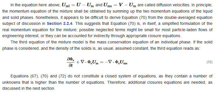
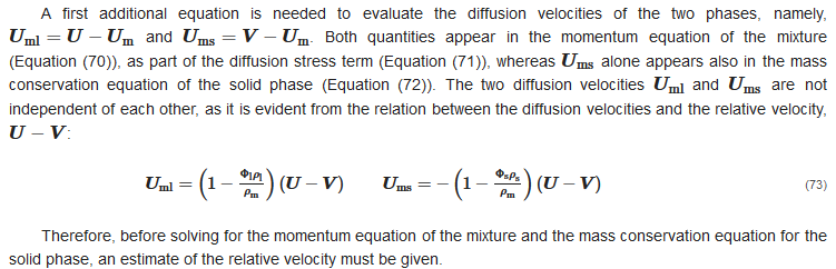
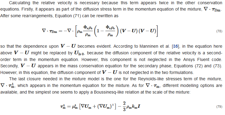
2.3.2. Closure Equations

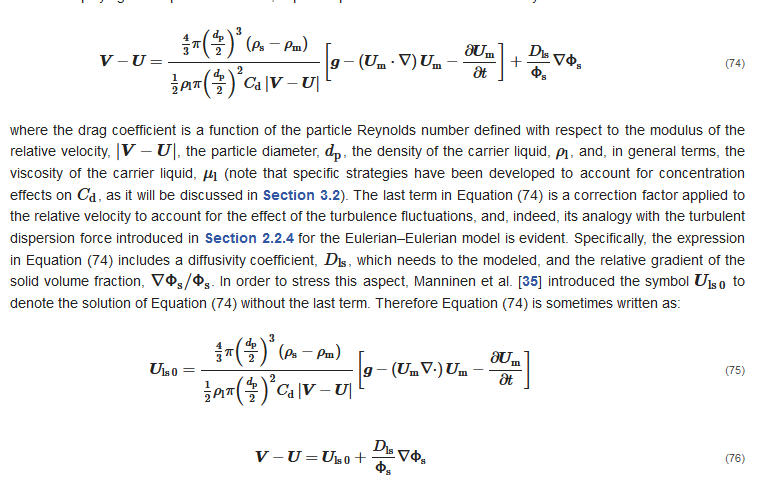
In the general formulation of Manninen et al. ^[34], the relative velocity is obtained by combining the momentum equation for the solid phase (Equation (66)) and the momentum equation of the mixture (Equation (70)), applying several simplifying assumptions. The final, implicit expression for the relative velocity reads as follows:

Although, strictly speaking, Equation (74) is a closure equation which accounts for the momentum transfer between the phases, it has sometimes been regarded as the last fundamental balance equation of the mixture model, alongside the mass conservation equation of the mixture (Equation (67)), the momentum conservation equation for the mixture (Equation (70)), and the mass conservation equation of the solid phase (Equation (72)). However, several other closures are required to close the system of the four equations.

For instance, for the viscous stresses in Equation (70), different modelling options are considered, but the simplest—yet commonly made—choice is to employ a Newton-like approximation made at the scale of the mixture, as follows,

Calculating the relative velocity is necessary because this term appears twice in the other conservation equations. Firstly, it appears as part of the diffusion stress term in the momentum equation of the mixture, ∇⋅τDm. After some rearrangements, Equation (71) can be rewritten as

2.3.3. Boundary Conditions

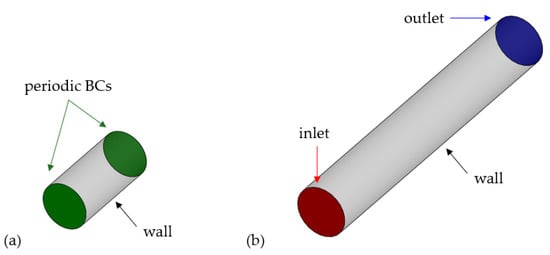
To the best of our knowledge, in all studies concerning the application of the mixture model to slurry pipe flows, the combination of inlet and outlet boundaries was employed (Figure 7b). At the inlet, the distributions of the solid volume fraction and of the velocity of the mixture are imposed, in addition to those of the turbulent parameters, such as $k_{m}$ and $ε_{m}$ . At the outlet, the pressure of the mixture is specified and held constant, and the normal gradient of all other variables are zero. At the solid walls, the same conditions of single-phase simulations are applied to the mixture. That is, a no-slip condition, which corresponds to zero advection flux from all surface cells; mixture-based wall functions to evaluate the mixture wall shear stress; different types of constraints for the turbulent parameters.

References

Derammelaere, R.H.; Shou, G. Altamina’s Copper and Zinc Concentrate pipeline incorporates advanced technologies. In Proceedings of the 15th International Conference on Hydrotransport, Banff, AB, Canada, 3–5 June 2002.
Paterson, A.J.C. Pipeline transport of high density slurries: A historical review of past mistakes, lessons learned and current technologies. Min. Technol. 2012, 121, 37–45.
van den Berg, C.H. IHC Merwede Handbook for Centrifugal Pumps and Slurry Transportation; MTI Holland: Kinderdijk, The Netherlands, 2013.
van Wijk, J.M.; Talmon, A.M.; van Rhee, C. Stability of vertical hydraulic transport processes for deep ocean mining: An experimental study. Ocean Eng. 2016, 125, 203–213.
Thomas, A.D.; Cowper, N.T. The design of slurry pipelines—Historical aspects. In Proceedings of the 20th International Conference on Hydrotransport, Melbourne, Australia, 3–5 May 2017.
Matoušek, V. Pressure drops and flow patterns in sand-mixture pipes. Exp. Therm. Fluid Sci. 2002, 26, 693–702.
Talmon, A.M. Analytical model for pipe wall friction of pseudo-homogenous sand slurries. Part. Sci. Technol. 2013, 31, 264–270.
Spelay, R.; Gillies, R.G.; Hashemi, S.A. Kinematic friction of concentrated suspensions of neutrally buoyant coarse particles. In Proceedings of the 20th International Conference on Hydrotransport, Melbourne, Australia, 3–5 May 2017.
Wilson, K.C. Deposition-limit nomograms for particles of various densities in pipeline flow. In Proceedings of the 6th International Conference on Hydraulic Transport of Solids in Pipes, Canterbury, UK, 26–28 September 1979.
Sanders, R.S.; Sun, R.; Gillies, R.G.; McKibbem, M.J.; Litzenberger, C.; Shook, C.A. Deposition velocities for particles of intermediate size in turbulent flow. In Proceedings of the 16th International Conference on Hydrotransport, Santiago, Chile, 26–28 April 2004.
Gillies, R.G.; Shook, C.A. Concentration distributions of sand slurries in horizontal pipe flow. Part. Sci. Technol. 1994, 12, 45–69.
Wilson, K.C.; Addie, G.R.; Sellgren, A.; Clift, R. Slurry Transport Using Centrifugal Pumps, 3rd ed.; Springer: New York, NY, USA, 2006.
Shook, C.A.; Gillies, R.G.; Sanders, R.S.; Spelay, R.B. Saskatchewan Research Council Course Notes; SRC Publications: Saskatoon, SK, Canada, 2013.
Menter, F. Two equation eddy-viscosity turbulence modeling for engineering applications. AIAA J. 1994, 32, 1598–1605.
Launder, B.E.; Spalding, D.B. Mathematical Models of Turbulence; Academic Press: London, UK, 1972.
Prosperetti, A.; Tryggvason, G. Computational Methods for Multiphase Flow; Cambridge University Press: New York, NY, USA, 2007.
Hager, A. CFD-DEM on Multiple Scales. An Extensive Investigation of Particle-Fluid Interactions. Ph.D. Thesis, Johannes Kepler University Linz, Linz, Austria, 2014.
Rettinger, C.; Godenschwager, C.; Eibl, S.; Preclik, T.; Schruff, T.; Frings, R. Fully resolved simulations of dune formation in riverbeds. In High Performance Computing; Kunkel, J.M., Yokota, R., Balaji, P., Keyes, D., Eds.; Springer: New York, NY, USA, 2017; pp. 3–21.
Peng, Z.; Doroodchi, E.; Luo, C.; Moghtaderi, B. Influence of void fraction calculation on fidelity of CFD-DEM simulation of gas-solid bubbling fluidized beds. AIChE J. 2014, 60, 2000–2018.
Zheng, E.; Rudman, M.; Kuang, S.; Chryss, A. Turbulent coarse-particle suspension flow: Measurement and modelling. Powder Technol. 2020, 373, 647–659.
Loth, E. Particle, Drops, and Bubbles. Fluid Dynamics and Numerical Methods; Draft for Cambridge University Press: 2010. Available online: www.academia.edu (accessed on 31 August 2021).
Elghobashi, S. On predicting particle-laden turbulent flows. Appl. Sci. Res. 1994, 52, 309–329.
Launder, B.E.; Spalding, D.B. The numerical computation of turbulent flows. Comput. Meth. Appl. Mech. Eng. 1974, 3, 269–289.
Huber, N.; Sommerfeld, M. Modelling and numerical calculation of dilute-phase pneumatic conveying in pipe systems. Powder Technol. 1998, 99, 90–101.
Breuer, M.; Alletto, M.; Langfeldt, F. Sandgrain roughness model for rough walls within Eulerian-Lagrangian predictions of turbulent flows. Int. J. Multiph. Flow 2012, 43, 157–175.
Burns, A.D.; Frank, T.; Hamill, I.; Shi, J.M. The Favre averaged drag model for turbulent dispersion in Eulerian multi-phase flows. In Proceedings of the 5th International Conference on Multiphase Flow, Yokohama, Japan, 30 May–4 June 2004.
Spalding, D.B. PHOENICS Encyclopedia. Models for Two-Phase Flows: Two-Equation k-ε Turbulence Model. Available online: http://www.cham.co.uk/phoenics/d_polis/d_enc/turmod/enc_tu74.htm (accessed on 22 July 2021).
Elghobashi, S.E.; Abou-Arab, T.W. A two-equation turbulence model for two-phase flows. Phys. Fluids 1983, 26, 931–938.
Mandø, M.; Lightstone, M.F.; Rosendahl, L.; Yin, C.; Sørensen, H. Turbulence modulation in dilute particle-laden flow. Int. J. Heat Fluid Flow 2009, 30, 331–338.
Messa, G.V.; Malavasi, S. Numerical prediction of dispersed turbulent liquid–solid flows in vertical pipes. J. Hydraul. Res. 2014, 52, 684–692.
Kaushal, D.R.; Thinglas, T.; Tomita, Y.; Kuchii, S.; Tsukamoto, H. CFD modeling for pipeline flow of fine particles at high concentration. Int. J. Multiph. Flow 2012, 43, 85–100.
Johnson, P.C.; Jackson, R. Frictional-collisional constitutive relations for granular materials, with application to plane shearing. J. Fluid Mech. 1987, 176, 67–93.
Messa, G.V.; Malavasi, S. Improvements in the numerical prediction of fully-suspended slurry flow in horizontal pipes. Powder Technol. 2015, 270, 358–367.
Manninen, M.; Taivassalo, V.; Kallio, S. On the Mixture Model for Multiphase Flow; VTT Technical Research Centre of Finland: Espoo, Finland, 1996.

© Text is available under the terms and conditions of the Creative Commons Attribution (CC BY) license; additional terms may apply. By using this site, you agree to the Terms and Conditions and Privacy Policy.

Upload a video for this entry

Information

Subjects: Engineering, Civil

Contributor MDPI registered users' name will be linked to their SciProfiles pages. To register with us, please refer to https://encyclopedia.pub/register :

Oluwaseun Adedeji

View Times: 1.1K

Update Date: 15 Sep 2021

Table of Contents

Video Upload Options

Confirm