Light detection and ranging (LiDAR)

Version	Summary	Created by	Modification	Content Size	Created at	Operation
1		Federica Villa	+ 3009 word(s)	3009	2021-06-09 11:36:06	\|
2	format correct	Karina Chen	Meta information modification	3009	2021-06-23 08:50:24	\|

This entry is adapted from the peer-reviewed paper 10.3390/s21113839

Light Detection and Ranging (LiDAR) is a 3D imaging technique, widely used in many applications such as augmented reality, automotive, machine vision, spacecraft navigation and landing. Achieving long-ranges and high-speed, most of all in outdoor applications with strong solar background illumination, are challenging requirements.

light detection and ranging (LiDAR) single photon avalanche diode (SPAD) silicon photo multiplier (SiPM) SPAD array time-of-flight (TOF) 3D ranging scanning

1. Introduction

Light detection and ranging (LiDAR) is a widespread technique used to reconstruct three-dimensional (3D) scenes for many applications such as augmented and virtual reality ^[1], automotive ^[2], industrial machine vision ^[3], Earth mapping ^[4], planetary science ^[5], and spacecraft navigation and landing ^[6]. Augmented reality is a leading branch, since it exploits applications in many fields such as vehicles navigation, military vision, flight training, healthcare and education. Many technology companies are pursuing great efforts in the automotive field for autonomous vehicles (AVs) and advanced driver assistance systems (ADAS), and the total available LiDAR market for ADAS, AV and trucks is expected to triple between 2025 and 2030, reaching up to USD120 B ^[7].

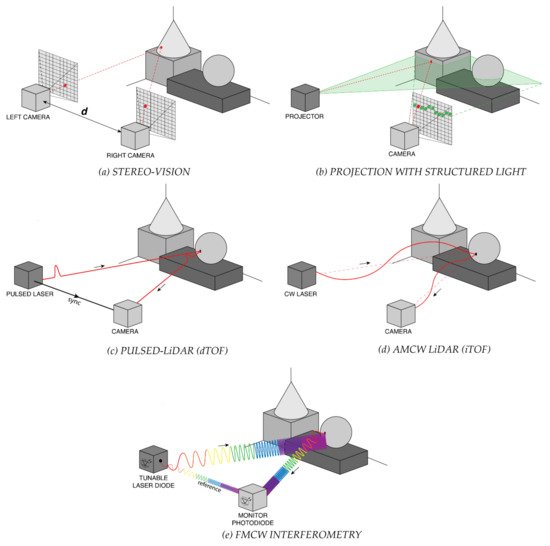
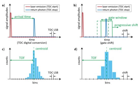
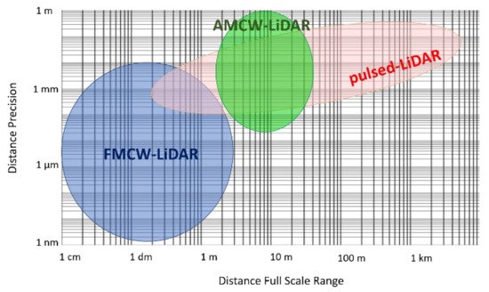
2. LiDAR Techniques

LiDAR techniques aim to reconstruct 3D maps of the environments under observation. Different methods for 3D ranging have been proposed, including stereo-vision, projection with structured light and time-of-flight (TOF), the latter being among the most promising one for long-range and real-time applications, and is commonly called LiDAR.

Triangulation exploits trigonometry laws to extract 3D spatial information ^[8]. In particular stereo vision ^[9] estimates distances through the simultaneous acquisition of two two-dimensional (2D) images of the same scene, by means of two cameras separated by a known distance d (Figure 1a). A sophisticated algorithm (named stereo disparity algorithm ^[10]) processes the images and computes the distance of the target. It is the same technique used by animals and humans to obtain information on distance and depth of objects in the surrounding environment. The advantage of stereo-vision is that it achieves high resolution and simultaneous acquisition of the entire range image in a simple passive-way, i.e., with neither active illumination nor energy emission. However, this method requires solving the so-called correspondence problem (identification of point pairs, which are projections of the same point in the scene), which is computationally expensive and results in a limited frame-rate ^[11]. Furthermore, stereo-vision is a non-robust technique, because of the parallax method used to measure distances. In fact, it fails if a nearby object covers a distant one in one of the two images; in that case, it is not possible to measure the further distance and the 3D image has a loss of information. The maximum Full-Scale-Range (FSR) depends on the baseline between the two cameras and the larger the base line the longer the range, but also the further the sensing range. Commercially available stereo vision cameras have typical operating distances of few meters (3 m to 5 m) ^[12]^[13]^[14].

Figure 1. Schematic representation of some 3D ranging techniques: (a) stereo-vision, (b) projection with structured light, (c) pulsed-LiDAR (dTOF), (d) amplitude-modulated continuous-wave (AMCW) LiDAR (iTOF), and (e) frequency-modulated continuous-wave (FMCW) interferometry.

Unlike stereo vision, projection with structured light requires an active illumination source, which shines a predetermined pattern of light (usually horizontal or vertical lines or spots, as shown in Figure 1b) toward the objects in the scene ^[15]. The 2D image is acquired and, analyzing how the light pattern gets modified by the targets, it is possible to reconstruct their 3D distance and shape. This technique is very accurate and precise (it can achieve sub-millimeter resolution), but it is slow because of the algorithm complexity, hence it cannot provide real-time acquisitions. Moreover, to improve depth resolution the pattern is changed several times (up to ten for every scene) and for each one the acquisition and the processing are repeated. The camera can also be moved around the scene, so to perform a high number of acquisitions, but lowering the overall measurement speed. For these reasons, structured light is used in applications where precision is a fundamental requirement instead of speed. Furthermore, the achievable FSR of commercially available structured light cameras is limited to few meters ^[16]^[17]^[18], which is another strong limitation in many applications. An example of commercial device based on structured light is the well-known Kinect v1 (Microsoft, Redmond, WA, USA) which can acquire 3D images with 5 mm precision up to 3.5 m range ^[19].

TOF techniques measure the path travelled by an excitation light through a medium to reach the target object and to return to the detector. They are widely exploited not only in LiDAR, but also in bioimaging ^[20]. Differently from stereo vision and structured-light projection, TOF-LiDAR does not require complex reconstruction algorithms, thus it enables real-time applications. Moreover, TOF techniques are the most suitable ones when large field of view (FOV) and centimeter resolution are needed. TOF can be directly measured, with time-resolved detectors and electronics (pulsed-LiDAR) or indirectly estimated through phase-resolved measurements (continuous wave or CW-LiDAR).

Pulsed-LiDAR, also known as direct-TOF (dTOF), relies on the measurement of the round-trip travel time of an optical pulse hitting and being back-scattered from a distant target (Figure 1c). From the TOF timing information, the distance D of the target is computed through the light velocity c in the medium, namely D = ½ · c · TOF. This technique requires short (usually <1 ns) laser pulses, high-bandwidth detectors and timing electronics with sub-nanosecond resolution and time jitter. In pulsed-LiDAR, the resolution of the electronics (σ_TOF) directly affects the depth resolution, being σ_d = ½ · c · σ_TOF. The distance FSR is only limited by the illuminator power, the target reflectivity and the timing electronics FSR. For this reason, pulsed-LiDAR is particularly suitable in applications requiring long ranges (up to kilometers).

In order to acquire long-range distances by employing low energy laser pulses and low reflectivity targets, single photon detectors together with photon-timing (e.g., a time-to-digital converter, TDC) and photon-counting (e.g., a digital gated counter) electronics become a must. In those cases, the laser return will no longer be an analog signal (e.g., photocurrent or photoelectron charge packet), but a digital pulse (e.g., a rising-edge logic transition when at least one photon gets detected). In the following we will mainly focus on these devices. In case of repetitive TOF measurements at the single-photon level, such technique is also known as time-correlated single-photon counting (TCSPC), able to reconstruct the shape of very faint and fast (down to the ps range) light signal ^[21], such as in fluorescence ^[22] and spectroscopy ^[23].

As shown in Figure 2, pulsed-LiDAR systems typically employ either TDCs to timestamp the arrival-time of the laser pulse echo (Figure 2a) or gated-detectors to measure the signal intensity within short gate windows, progressively spanning across the FSR with increasing gate delays from the laser pulse emission (Figure 2b). Both techniques can be applied also with very dim signals at single photon rate, repeating many times the measurements in order to build a histogram of the acquired data (either TOFs or intensities), whose bin-width depends on either TDC resolution or gate window delay shift, respectively (Figure 2c,d). Each measurement can look at a single spot of the scene or at the full scene, depending on the optics and if a single-pixel detector or a multi-pixel imager is employed; anyhow, usually a histogram is accumulated per each pixel. The computation of the histogram centroid gives the average TOF, hence the distance of the spatial spot imaged by the LiDAR’s optics. Thus information about the target distance and shape can also be extracted from the histogram of the reflected signal.

Figure 2. Schematic representation of different pulsed-LiDAR approaches: (a) a TDC measures the arrival-time of incoming photons (the time axis is quantized by the TDC’s Least Significant Bit, LSB); (b) a gated-detector measures the signal intensity within a gate window that is progressively-scanned across the range (the time axis is quantized by the gate shifts). In both cases, the histogram of collected data, either TDC timing information (c) or measured intensities (d), is used to extract the distribution centroid, corresponding to the average TOF.

The TDC approach is sensitive to all photons returning within the FSR, whereas the gated-detector approach counts only photons returning within the selected gate window, with the advantage of time filtering the incoming light and reduce the distortion due to background illumination. On the other hand, time-gating drastically reduces the actual detection efficiency of the measurement, therefore, progressive-scanning requires long measurement times regardless of the background conditions, and it results hardly compatible with real-time applications and long ranges. Vice versa, the TDC approach could be limited by either the maximum number of TDC conversions and storage availability per laser pulse or the dead-time of both TDC and single-photon detector (i.e., the time required to be ready for a next conversion or detection). Therefore, compared to the ideal case of 100% detection efficiency, no dead-times, multi-hit TDC electronics, actual pulsed-LiDAR systems may have major performance limitations.

In continuous-wave CW-LiDAR, instead of emitting short high-energy laser pulses, either amplitude modulated (AMCW) or frequency modulated (FMCW) light is employed. AMCW-LiDAR is achieved through the so-called indirect-TOF (iTOF) technique, which relies on measurement of the phase difference between an amplitude modulated light source and the detected backscattered echo signal (Figure 1d). The excitation signal can be either a sinusoidally amplitude modulated light or a light pulse (with hundreds of nanoseconds pulse width) from lasers or LEDs. In the sinusoidal modulation approach, the echo signal is phase-shifted with respect to the emitted one, by a quantity proportional to the source modulation frequency f and the object distance. From the phase shift ΔФ, it is then possible to infer the distance D = c ∙ΔΦ/4πf. Usually ΔФ is measured by sampling the sinusoidal echo intensity in four equally spaced points (C₀, C₁, C₂ and C₃) and by computing \( \Delta\Phi=arctg\left(\frac{C3-C1}{C0-C2}\right) \) [24].

In the pulsed modulation approach, a laser source emits light pulses with duration T_p of few hundreds of nanoseconds (usually proportional to the desired FSR) and the back-scattered light is integrated within three time windows, with same width but delayed in time. The first one integrates the whole signal (background plus echo pulse), the second one integrates the same background but only a portion of the echo pulse; the third time window integrates just the background light, which is then subtracted from the two previous measurements. The ratio between the two resulting intensities (multiplied by 2π) provides the phase shift ΔФ. In this way, the measurement is independent of background light, illumination power and object reflectivity, while in AMCW-LiDAR the resolution strongly depends on all of them. Eventually, the distance is computed as \( D=\frac12\cdot T_p\cdot \left(1-\frac{\Delta \Phi}{2\pi}\right) \)^[24]. Usually, the FSR is limited by the modulation period: e.g., 100 ns pulses or 10 MHz modulation allow to reach 100 ns FSR, i.e., 15 m distance. Nevertheless, methods based on multiple modulation frequencies or linearly chirped modulations have been implemented to extend the unambiguous measurement range ^[25].

In frequency-modulated FMCW-LiDAR, the laser frequency (i.e., the laser wavelength) is modulated. Typically, the modulation consists of a linear chirp with a small portion of the laser beam (reference) used as local oscillator for the heterodyne demodulation of the return echo signal, as shown in Figure 1e. The modulation bandwidth is often wider than the linearly-chirped AMCW-LiDAR one, yielding to improved depth resolution ^[26]. Detection requires an optical heterodyne measurement to exploit the interference between emitted and backscattered optical waves, for example through a standard or p-i-n photodiode to demodulate the return signal and generate a beat frequency, which can be recorded by “slow” electronics. The achievable precision is typically much better than in pulsed-LiDAR (dTOF), with the major advantage of using low-bandwidth electronics and cost-effective detectors. Another advantage of FMCW-LiDAR is its ability to directly measure the velocity of the target object by extracting the Doppler-shift generated from the motion ^[27]. The main limitation of FMCW-LiDAR is the demanding long coherence length of the laser, as it influences the stability of the local oscillator in respect to the backscattered wave, introducing phase-noise. If the measured distance is shorter than the laser coherence length, the peak of the beat-frequency spectrum results sharp and narrow, otherwise the peak widens and its amplitude decreases. Thus the laser coherence length limits the achievable distance FSR. However, FMCW-LiDAR systems able to reach up to 300 m distance range have been recently announced by different companies for automotive applications ^[28]^[29].

Only LiDAR techniques can reach long ranges, since both stereo-vision and structured-light approaches are limited to few meters. Figure 3 shows the typical trade-off between precision and FSR of pulsed-LiDAR, AMCW-LiDAR and FMCW-LiDAR systems published starting from 1990 ^[11]. We can observe that FMCW-LiDAR allows to reach the best precision, but typically at short ranges. Recent commercial FMCW-LiDAR systems which reach long-ranges (up to 300 m) ^[28]^[29] have not been reported in Figure 3 since the achieved distance precision is never mentioned. Pulsed-LiDAR is the only one reaching long distances (up to few kilometers) in real-time, a mandatory requirement in many fields such as automotive. For this reason, in this paper we will mainly focus on pulsed-LiDAR (dTOF) systems at the single-photon level.

Figure 3. Typical distance Precision vs. Full-Scale Range in pulsed-LiDAR, AMCW-LiDAR and FMCW-LiDAR systems reported so far. Figure adapted from ^[11].

3. Illumination Schemes

TOF-LiDAR techniques require to illuminate the scene by means of either a single light spot, a blade beam, or a flood illumination, as shown in Figure 4. The former two need to cover the whole scene through respectively 2D or 1D scanning, whereas the latter is exploited in flash-LiDAR with no need of scanning elements.

Single-spot illumination typically employs also a single pixel detector (Figure 4-a); hence, a coaxial optical system (as shown in Figure 4-f) is preferred, in order to avoid any alignment and parallax issue. Note that such a single pixel may be composed by a set (e.g., an array) of detectors, all acting as an ensemble detector (i.e., with no possibility to provide further spatial information within the active area), such as in Silicon PhotoMultipliers. Alternatively, it is also possible to use a 2D staring array detector (with an active area larger than the laser spot), shining the illumination spot onto the target through a simple non-coaxial optical setup, and eventually measuring the signal echo which walk across the 2D detector, depending also on the object distance (Figure 4-b). The main disadvantage is a lower Signal-to-Noise Ratio (SNR) because the detector collects the laser echo from the target spot but also the background light from a larger surrounding area. A more complex detector architecture or readout electronics can recover the ideal SNR by properly tracking the laser spot position within the 2D array detector, so to discard off-spot pixels, for example as proposed in [31].

Blade illumination can be employed in combination with linear detector arrays, mechanically spinning around their axis so to speed up scanning, or using a co-axial optical system (Figure 4-c) such as in the Velodyne LiDAR system [32]. Also in this case, it is possible to scan only the blade illumination, while keeping fixed a 2D staring array detector imaging the overall scene, or activating only one row at a time (Figure 4-d).

Finally, flash-LiDAR relies on a flood illumination of the whole scene, while using a staring camera where each pixel images one specific spot of the scene and measures the corresponding distance (Figure 4-e). The name “flash” highlights the possibility to acquire images at very high framerates, ideally also in a single laser shot, since no scanning is needed. However, the required laser pulse energy is typically extremely high for covering a sufficiently wide FOV, often far exceeding the eye-safety limits in case of human crossing the FOV at very short distance.

When scanning is required, the beam-steering can be performed with either optomechanical elements (e.g., rotating mirrors and prisms) and electromechanical moving parts (e.g., electric motors with mechanical stages) or compact Micro Electro-Mechanical Systems (MEMS) mirrors and solid-state Optical Phase Arrays (OPAs). MEMS and OPAs offer a more compact and lightweight alternative to electromechanical scanning and consequently also faster scanning, for instance through the usage of resonant mirrors. MEMS technology is by far more mature than OPAs, so to become the most exploited technology in modern LiDAR scanning systems [33].

The selection of the illumination scheme must trade off many parameters, such as laser energy, repetition frequency, eye-safety limits, detector architecture, measurement speed, and system complexity. Indeed, compared to scanning techniques, flood illumination in flash-LiDAR typically requires higher laser power to illuminate the entire scene in one shot and assuring enough signal return onto the detector. Such flood illumination could be convenient for eye-safety considerations (if no human being stays too close to the LiDAR output port) because, even if the total emitted power is high, it is spread across a wider area, so the power for unit area could be lower than single-spot long-range illumination. Flash-LiDAR has the advantage of simpler optics, at the expense of large pixel number 2D detector. In fact, the number of pixels limits the angular resolution given the FOV, or vice versa limits the FOV given the angular resolution. Instead, scanning negatively impacts acquisition speed and framerate: particularly 2D scanning is very slow and hardly compatible with real-time acquisitions and fast-moving targets. However, also flash-LiDAR can be operated not single-shot but with more laser shots and image acquisitions to collect enough signal, because the total pulse energy is distributed across a wide FOV and the return signal (above all from far-away objects) can be extremely very faint. In the following, we will focus on both 1D linear scanning with blade illumination and flash-LiDAR with flood illumination, because there is no preferred one for all applications.

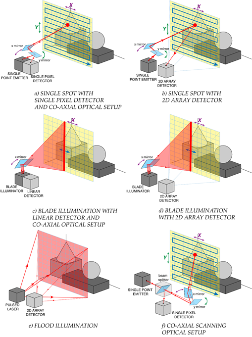
Figure 4. TOF-LiDAR illumination schemes: (a) 2D raster scan with single spot and one pixel detector in a co-axial optical setup, (b) 2D raster scan with single spot and a 2D array detector, (c) 1D line scan with blade beam and a linear array detector in a co-axial optical setup, (d) 1D line scan with blade beam and a 2D array detector, (e) no scan with flood illumination and 2D imager (full scene flash acquisition), for flash-LiDAR. (f) Example of a co-axial scanning optical setup.

References

Bronzi, D.; Zou, Y.; Villa, F.; Tisa, S.; Tosi, A.; Zappa, F. Automotive Three-Dimensional Vision through a Single-Photon Counting SPAD Camera. IEEE Trans. Intell. Transp. Syst. 2016, 17, 782–785.
Warren, M.E. Automotive LIDAR Technology. In Proceedings of the Symposium on VLSI Circuits, Kyoto, Japan, 9–14 June 2019; pp. C254–C255.
Steger, C.; Ulrich, M.; Wiedemann, C. Machine Vision Algorithms and Applications; Wiley: Hoboken, NJ, USA, 2018.
Glennie, C.L.; Carter, W.E.; Shrestha, R.L.; Dietrich, W.E. Geodetic imaging with airborne LiDAR: The Earth's surface revealed. Rep. Prog. Phys. 2013, 76, 086801.
Yu, A.W.; Troupaki, E.; Li, S.X.; Coyle, D.B.; Stysley, P.; Numata, K.; Fahey, M.E.; Stephen, M.A.; Chen, J.R.; Yang, G.; et al. Orbiting and In-Situ Lidars for Earth and Planetary Applications. In Proceedings of the IEEE International Geoscience and Remote Sensing Symposium, Waikoloa, HI, USA, 26 September–2 October 2020; pp. 3479–3482.
Pierrottet, D.F.; Amzajerdian, F.; Hines, G.D.; Barnes, B.W.; Petway, L.B.; Carson, J.M. Lidar Development at NASA Langley Research Center for Vehicle Navigation and Landing in GPS Denied Environments. In Proceedings of the IEEE Research and Applications of Photonics In Defense Conference (RAPID), Miramar Beach, FL, USA, 22–24 August 2018; pp. 1–4.
Rangwala, S. Lidar: Lighting the path to vehicle autonomy. SPIE News, March 2021. Available online: (accessed on 31 May 2021).
Hartley, R.I.; Sturm, P. Triangulation. Comput. Vis. Image Underst. 1997, 68, 146–157.
Bertozzi, M.; Broggi, A.; Fascioli, A.; Nichele, S. Stereo vision-based vehicle detection. In Proceedings of the IEEE Intelligent Vehicles Symposium, Dearborn, MI, USA, 5 October 2000; pp. 39–44.
Sun, J.; Li, Y.; Kang, S.B.; Shum, H.Y. Symmetric Stereo Matching for Occlusion Handling. In Proceedings of the IEEE Computer Society Conference on Computer Vision and Pattern Recognition, San Diego, CA, USA, 20–25 June 2005; Volume 2, pp. 399–406.
Behroozpour, B.; Sandborn, P.A.M.; Wu, M.C.; Boser, B.E. Lidar System Architectures and Circuits. IEEE Commun. Mag. 2017, 55, 135–142.
ENSENSO XR SERIES. Available online: (accessed on 25 May 2021).
Structure Core. Available online: (accessed on 25 May 2021).
Intel® RealSense™ Depth Camera D455. Available online: (accessed on 25 May 2021).
Geng, J. Structured-light 3D surface imaging: a tutorial. Adv. Opt. Photon. 2011, 3, 128–160.
PRIMESENSE CARMINE. Available online: (accessed on 25 May 2021).
Structure Sensor: Capture the World in 3D. Available online: (accessed on 25 May 2021).
Atra ORBBEC. Available online: (accessed on 25 May 2021).
Smisek, J.; Jancosek, M.; Pajdla, T. 3D with Kinect. In Consumer Depth Cameras for Computer Vision; Springer: Berlin, Germany, 2013; pp. 3–25.
Hansard, M.; Lee, S.; Choi, O.; Horaud, R.P. Time-of-Flight Cameras: Principles, Methods and Applications; Springer: Berlin, Germany, 2012.
Becker, W. Advanced Time-Correlated Single Photon Counting Techniques; Springer: Berlin, Germany, 2005.
Becker, W.; Bergmann, A.; Hink, M.A.; König, K.; Benndorf, K.; Biskup, C. Fluorescence lifetime imaging by time-correlated single-photon counting. Microsc. Res. Tech. 2004, 63, 58–66.
Becker, W.; Bergmann, A.; Kacprzak, M.; Liebert, A. Advanced time-correlated single photon counting technique for spectroscopy and imaging of biological systems. In Proceedings of the SPIE, Fourth International Conference on Photonics and Imaging in Biology and Medicine, Tianjin, China, 3–6 September 2005; p. 604714.
Bronzi, D.; Zou, Y.; Villa, F.; Tisa, S.; Tosi, A.; Zappa, F. Automotive Three-Dimensional Vision through a Single-Photon Counting SPAD Camera. IEEE Trans. Intell. Transp. Syst. 2016, 17, 782–785.
Bellisai, S.; Bronzi, D.; Villa, F.; Tisa, S.; Tosi, A.; Zappa, F. Single-photon pulsed light indirect time-of-flight 3D ranging. Opt. Express 2013, 21, 5086–5098.
Zhang, C.; Zhang, Z.; Tian, Y.; Set, S.Y.; Yamashita, S. Comprehensive Ranging Disambiguation for Amplitude-Modulated Continuous-Wave Laser Scanner With Focusing Optics. IEEE Trans. Instrum. Meas. 2021, 70, 8500711.
Lum, D.J.; Knarr, S.H.; Howell, J.C. Frequency-modulated continuous-wave LiDAR compressive depth-mapping. Opt. Express 2018, 26, 15420–15435.
Zhang, F.; Yi, L.; Qu, X. Simultaneous measurements of velocity and distance via a dual-path FMCW lidar system. Opt. Commun. 2020, 474, 126066.
FMCW Lidar: The Self-Driving Game-Changer. Available online: (accessed on 25 May 2021).
Radar & LiDAR Autonomous Driving Sensors by Mobileye & Intel. Available online: (accessed on 25 May 2021).

© Text is available under the terms and conditions of the Creative Commons Attribution (CC BY) license; additional terms may apply. By using this site, you agree to the Terms and Conditions and Privacy Policy.

Upload a video for this entry

Information

Subjects: Engineering, Electrical & Electronic

Contributor MDPI registered users' name will be linked to their SciProfiles pages. To register with us, please refer to https://encyclopedia.pub/register :

Federica Villa

View Times: 1.6K

Update Date: 23 Jun 2021

Table of Contents

Video Upload Options

Confirm

1. Introduction

2. LiDAR Techniques

3. Illumination Schemes

References