Graph Modeling of Shop Schedulings

Version	Summary	Created by	Modification	Content Size	Created at	Operation
1		Golshan Madraki	+ 21809 word(s)	21809	2021-05-24 06:38:14	\|
2	format correct	Conner Chen	-12650 word(s)	9159	2021-05-25 10:40:01	\|

This entry is adapted from the peer-reviewed paper 10.3390/app11114741

Graphs are powerful tools to model manufacturing systems and scheduling problems. The complexity of these systems and their scheduling problems has been substantially increased by the ongoing technological development. Thus, it is essential to generate sustainable graph-based modeling approaches to deal with these excessive complexities. Graphs employ nodes and edges to represent the relationships between jobs, machines, operations, etc. Despite the significant volume of publications applying graphs to shop scheduling problems, the literature lacks a comprehensive survey study. We proposed the first comprehensive review paper which 1) systematically studies the overview and the perspective of this field, 2) highlights the gaps and potential hotspots of the literature, and 3) suggests future research directions towards sustainable graphs modeling the new intelligent/complex systems. We carefully examined 143 peer-reviewed journal papers published from 2015 to 2020. About 70% of our dataset were published in top-ranked journals which confirms the validity of our data and can imply the importance of this field. After discussing our generic data collection methodology, we proposed categorizations over the properties of the scheduling problems and their solutions. Then, we discussed our novel categorization over the variety of graphs modeling scheduling problems. Finally, as the most important contribution, we generated a creative graph-based model from scratch to represent the gaps and hotspots of the literature accompanied with statistical analysis on our dataset. Our analysis showed a significant attention towards job shop systems (56%) and Un/Directed Graphs (52%) where edges can be either directed, or undirected, or both. Whereas 14% of our dataset applied only Undirected Graphs, and 11% targeted hybrid systems, e.g., mixed shop, flexible and cellular manufacturing systems which shows potential future research directions.

graph theory shop scheduling problem Modeling Manufacturing systems A systematic review and categorization methodology

1. Introduction

Graph theory is an important and practical division in mathematics. It is defined as the study of graphs which are a visual representation and a mathematical structure showing the relations between elements and/or features of a problem (^[1]. Graphs have two major components: nodes (also known as vertices and points) and edges (also known as links, lines, arrows) connecting nodes together, dictating the relationship between nodes. Edges can be directed or undirected. If a node takes precedence over another node, then this relation is represented by a directed edge. otherwise, an undirected edge should be used connecting two symmetric nodes.

Graph theory was first published in 1735 by Euler with the solution of the Königsberg bridge problem ^[2]. Euler turned land masses into nodes and bridges into undirected edges, finding that his solution depended on a characteristic of the graph: the degrees of each node. Rather than simplifying this problem, Euler’s method clarified the problem into only the necessary components and relationships for understanding and solving. Since 1735, graph theory has expanded vastly in both applications and complexity. Today, graph theory includes hundreds of different types of graphs, algorithms, heuristics, and accompanying mathematical structures.

The major application of graph theory is to model a variety of problems across disciplines and industries in which networks exist including physics ^[3]^[4], computer science ^[5]^[6], social networks ^[7]^[8], political science ^[9], artificial intelligence ^[10], biology ^[11], electrical power systems ^[12]^[13]^[14], supply chain network ^[15]^[16], we well as global crisis research such as COVID-19 outbreak ^[17].

Manufacturing systems benefit greatly from graph theory because they are all, at a fundamental level, networks of assets processing materials, parts, and information ^[18]. With this knowledge, they can be converted into graphical models efficiently and then analyzed.

Shop scheduling is a critical subsystem of control and planning process in manufacturing systems, and directly affects the system productivity. Shop scheduling problems have been profoundly studied within the past decades. Scheduling generally refers to the assignment of a set of jobs to a set of resources (usually machines) within the course of time. As the size of sets of jobs and machines gets larger, finding a feasible schedule becomes harder. The ultimate goal in a scheduling problem is to find an efficient schedule which yields optimal results for the designated system performance measure/s (objective/s) ^[19].

2. The Theory of Shop Scheduling Problems

Shop Scheduling problems (also known as manufacturing system scheduling) are well-known optimization problems in the field of operations research ^[20]^[21]. Understanding the concepts and the characteristics of manufacturing systems is essential to efficiently model the associated scheduling problems. Thus, in this section, we will review and classify different manufacturing systems and scheduling problems.

In a manufacturing system, there might be multiple jobs that should be processed by multiple machines. Processing a job by a machine is called an operation or task. The order in which machines process jobs is known as the machines’ schedule ^[22]^[23]^[24]. Finding an appropriate machines’ schedule which results in desired values for performance measures is called as Scheduling Problem ^[25]^[22]^[26]. Ideally, an optimal performance measure is reached through the optimal schedule. Almost all shop scheduling problems are NP-hard. There are a few simple versions of flow shop scheduling problems that can be solved optimally in 0(nlog_n) where n is the number of operations.

The common terminology in the field of shop scheduling problem is listed in Table 1. Some of the terms refer to constraints or specific situations. Depends on the problem definitions/requirements, experts may incorporate some of these items into the problem.

Table 1. Common terminology in Manufacturing system and shop scheduling problems.

Term	Description
Buffer	A waiting space for jobs between machines. Buffers avoids blocking situation
Blocking	This situation occurs when a machine cannot release a job due to lack of buffer. It halts further tasks until the buffer is restored
Start Time (S_ij)	The time when job j starts being processed by machine i.
Processing Time (Pij)	is the time it takes for machine i to process job j
Travel Time	The time for a job to be transferred from one machine to another
Setup Time	The time required to prepare a system or machine for production
Bottleneck	The process that directly limits production capacity, i.e., the critical path.
Dispatching	Assigning resources to tasks, i.e., scheduling.
Assembly	A product of combined components.
Subassembly	A component that is built by combining several other components and used in a larger product.
Precedence	Job j can only start processing after jobs in set s have been completed.
Machine Eligibility	Machine i can only perform some subset of job j’s required processes.
Machine Breakdown	Machines have non-continuous availability.
Routing	Job j’s operations must be completed in a specific order.
Incompatible jobs	Incompatible jobs cannot be processed by the same machine
Waiting Time	This situation occurs when the buffer between machines is too small blocking may occur, so, upstream machines cannot release jobs.
No-Wait	Consecutive operations of a job must be performed without wait-time on either machine.
No-Idle	Machines must continuously process jobs without overlap or pause.
Deadlock	This situation occurs when the order of operations creates a cycle, and the entire process stops under this situation.
Preemption	Jobs can be interrupted while being processed on machines. They can then be resumed on the same machine or a new one.

2.1. Objectives of Scheduling Problems

Different objective functions or performance measures are used in the scheduling problems. Makespan is the most common and the popular measure one which refers to the completion time of all operations of all jobs in the systems.

Table 2 shows the list of commonly used performance measures followed by their definition.

Table 2. Commonly used objective (performance measure) in different manufacturing systems.

Objective	Description
Makespan	Total completion time: the time taken to complete all jobs.
Total workload of Machines	The total processing time across all machines.
Workload of most loaded machine	The machine(s) with the largest processing time(s).
Max lateness	The largest difference between a given job’s completion time and deadline.
Mean flow time	The average amount of time that a given job spends on the shop floor.
Tardiness	The difference between a given job’s completion time and deadline.
Total tardiness	The sum of each job’s tardiness.
Mean tardiness	The average of all jobs’ tardiness.
Weighted tardiness	The difference between a given job’s completion time and deadline multiplied by a weight (corresponding to cost).

2.2. Shop Layouts

A very basic layout of all manufacturing systems includes a finite number of jobs, machines where J and M denotes the set of jobs and the set of machines, respectively; and 0 is the set of operations/tasks. A route (also known as the sequence) refers to the order of machines that a job should passes through ^[22]^[27]^[28]. Manufacturing systems and their layouts may be distinguished by their uniformity, existence of fixed routes, the flexibility of machines, the number of machines, and existence of buffer, set up times, etc. These differences come from variations in demand and required levels of production flexibility ^[29].

Baker ^[30] was a pioneer proposing a classification of classical manufacturing systems and their associate scheduling problems into the single-stage production system and multi-stage systems. In his classification, single-machine and parallel-machine are the single-stage layouts, and job shop, flow shop, and open shop systems are the classical multi-stage layouts.

We utilized classical classifications and modern models as well as different scholars’ literature review studies to propose our comprehensive classification of system layouts as it is represented in Figure 1. In addition to the classical layouts, we incorporated the modern complicated layouts such as mixed shop and just-in-time systems in our classification. These modern system layouts emerged during the recent decades to satisfy the needs of fast-growing manufacturing technology.

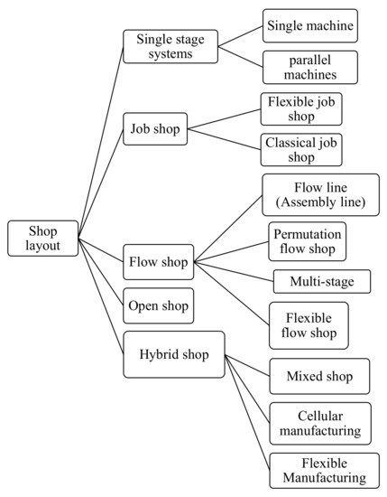
Figure 1. Shop layout classification.

In this section, the main properties of each layout are briefly explained. Reviewing this background is particularly important to understand how different types of graphs can be applied to address scheduling problems in different manufacturing structures.

2.2.1. Single-Stage System

The simplest manufacturing layout is the single-stage system where there is only one work-center and a set of identical jobs passing through this work-center. The work-center may contain only a single machine or multiple machines.

A scheduling problem for a single machine system may be defined when all jobs are not available at the beginning of the process but instead jobs are given release dates or alternatively, a distinct due window is defined for each job ^[31]. A scheduling problem for a single machine system may be defined when all jobs are not available at the beginning of the process but instead jobs are given release dates or alternatively, a distinct due window is defined for each job ^[31].

When there are multiple machines in the single stage system, all machines should be arranged in parallel fashion. The multiple parallel machines can be either identical machines, or similar machines with different speeds (uniform parallel machines), or unrelated parallel machines ^[32]^[33]^[34]. Many single stage scheduling problem can be solved in polynomial-time ^[32].

2.2.2. Job Shop System

Job shops (JS) are well-known manufacturing systems built for high flexibility and a wide range of applications. Machines within a classic job shop are fixed, unique, meaning they only have the capability of processing one type of operation, and may only process one operation at a time. All machines are available at time zero. Each job is independent of another and can follow a unique path through the machines to fulfill all operations, meaning routes of different jobs are not uniform. All jobs are available after release dates and operations cannot be interrupted.

The job shop scheduling problem (JSSP) is a frequent topic of research due to its NP hardness ^[35]. To model systems resembling realistic shop floors, the classic JSSP has been widely expanded upon with the additions of constraints such as blocking, introducing a zero-buffer capacity, ^[36]^[37]^[38], no-wait, and no-idle. Classic JSSP has also been expanded to account for distributed work centers, creating the distributed JSSP ^[39]. To model systems resembling realistic shop floors, the classic JSSP has been widely expanded upon with the additions of constraints such as blocking, introducing a zero buffer capacity, ^[36]^[37]^[38], and no-wait, meaning consecutive operations of a job must be performed without wait-time on either machine, ^[40]. Classic JSSP has also been expanded to account for distributed work centers, creating the distributed JSSP ^[39]. To model systems resembling realistic shop floors, the classic JSSP has been widely expanded upon with the additions of constraints such as blocking, introducing a zero buffer capacity, ^[36]^[37].

Machines in a flexible job shop (FJS) may have the capability of doing more than one type of operation. The classic JSSP can be expanded to include this new attribute, creating the flexible JSSP ^[41]. While increasing flexibility, the inclusion of this attribute increases the complexity as well ^[42]. Flexible JSSP must now include the assignment of operations to capable machines as the first step, compared to previously classic JSSP assumed a predefined route for each job and a single option of machine to complete a given operation ^[43]. After that assignment, then flexible JSSP works similarly to JSSP such that a feasible and ideally optimal schedule is found based on predetermined objectives ^[19].

The flexible JSSP can be broken down into two subcategories: still including the concept of a predefined route for a given job (operations must be done in a certain sequence), or removing that concept and introducing alternative routes ^[44].

Flexible JSSP may come in many names. Such that JSSP with multi-purpose machines, ^[45], multi-processor JSSP ^[46], and JSSP with unrelated parallel machines ^[47].

2.2.3. Flexible Manufacturing System (FMS)

A flexible manufacturing system (FMS) is a relatively new technology which refers to an automated hybrid of flexible job shop ^[48] which utilizes an automated material handling system to maneuver jobs between machines ^[49]. All machine and material handling systems are monitored and controlled by a centralized computer ^[50].

The FMS scheduling problem resembles JSSP with some extensions including the movements of the material handling system and its common constraints of blocking and holdup ^[48].

Common objectives within the FMS scheduling problem include makespan, mean flowtime, and maximum flowtime ^[49]. Often additional objectives will be included regarding the travel time within the material handling system ^[51].

2.2.4. Flow Shop System

At the opposite end of flexibility, flow shop (FS) is another well-known manufacturing system. FS features a number of machines; each machine performs a single process on jobs that flow through in a unidirectional fashion ^[52].

Note that FS do possess a degree of flexibility as it can process different jobs simultaneously (although machines can only perform one task on one job at a time) and jobs are not required to be processed by each machine in the sequence ^[52]. Additionally, jobs may be allowed to have different completion times, instead of strictly being uniform ^[52].

The flow shop scheduling problem (FSSP) often looks to minimize makespan, total flowtime, tardiness, idle time, and other performance measures to ideally find an optimal schedule ^[53]. While not NP-hard by default, FSSP can become NP hard with a sufficient number of constraints, batch size, and number of machines ^[54].

The simplest and the most common version of FS is when the order of machines for all jobs are predetermined and fixed, and the modifiable element is the schedule of jobs on machines ^[55]. The flow line (also known as assembly line) is a subcategory of FS with less flexibility and more effectiveness and speed (due to its simplicity). Unlike FS, flow line requires all jobs to be identical ^[56]. Added complexity to a flow line scheduling problem is often variation in processing time of machines. Understanding the structure of the flow lines is particularly important since some scheduling problems in literature are defined as hybrid layouts featuring sections of flow lines. For example, an assembly-type FS is a hybrid production system featuring production areas arranged as a JS to produce component parts. These components or subassemblies are fed into a flow line arranged as a FS for final assembly operations ^[57]^[58].

Within FS, jobs often follow similar routes or are identical, as in flow line. When jobs are processed in the same order on every machine, meaning their routes are identical, a permutation schedule is developed ^[59]^[60]. A FS in which this type of schedule occurs is known as permutation flow shop. The processing times on a machine may vary from job to job.

The flexible flow shop (FFS) consists of multiple stages. One or more parallel machines are available in each stage, but at least one of these stages includes multiple machines ^[34]. This system allows jobs to “skip” stages if they are not necessary ^[61]^[62].

2.2.5. Open Shop

The layout of open shop systems is like job shop systems, i.e., a set of jobs should be processed by a set of machines. However, the order of machines that each job should pass through or the order in which the processing steps of a job take place is arbitrary and can alternate freely. This important feature allows a greater number of possible job flow permutations leading it to be significantly harder from a computational standpoint ^[63].

The goal of the open shop scheduling problem is to find an appropriate order of assignment of jobs to machines to optimize some performance measures (e.g., makespan). In this solution, a job cannot be assigned to two machines at the same time; and a machine cannot process two jobs at the same time ^[64]^[65]^[66].

2.2.6. Mixed Shop

A mixed shop system (in some cases known as hybrid shop ^[19]) can include any combination of classical shop system such as open shop and job/flow shop ^[67]. Within mixed shop system, some jobs have predefined routes, like job shop or flow shop, while some jobs do not, like open shop ^[67]. Also, an operation for a job might need a set of machines instead of a single machine. This set of machines must process simultaneously and in sequence fashion ^[19].

Mixed shop is well known for its capability to resemble real-world complex systems. Custom or semi-custom manufacturing systems widely use mixed shop structure since some operations are very complicated and might require multiple simultaneous processing steps (by either operators or machines) ^[19]^[68].

The complexity of the mixed shop scheduling problem depends heavily on whether the operations per job is unlimited or not ^[67].

2.2.7. Cellular Manufacturing System (CMS)

The cellular manufacturing systems (CMS) have been introduced as an efficient layout in the philosophy of just-in-time and lean manufacturing which concerned with optimizing processes for time and value. To meet increasing demand for mid-volume and mid-diversity product mixes, CMS is designed as a hybrid of job shops and flow lines. CMS have cells containing grouped machines (or operators, workstations, etc.) that process jobs ^[69]^[70]. Jobs are grouped in part-families and ideally do not leave their cell ^[69].

The scheduling of cellular manufacturing is often referred to as flow shop group scheduling ^[71] and sometimes distinguishes inter-cell scheduling from intra-cell scheduling ^[69]^[72]. The scheduling problem includes cell formation, assigning machines to each cell, and general task scheduling ^[73].

3. Classifications and Solutions of Scheduling Problems

Scheduling consists of allocating given tasks to given resources over a period of time ^[74]. The theory behind scheduling is to create an efficient allocation and has many applications across industries ^[75]. Specifically efficient production scheduling is key to manufacturing performance and productivity ^[76]. Once manufacturing context has been set, scheduling solutions can be found in many ways.

3.1. Classification of Scheduling Problems

Lin, Gen ^[77] proposed a popular classification of scheduling problems based on their processing characteristics as represented in Figure 2.

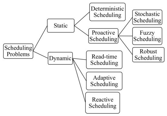
Figure 2. Lin, Gen ^[77] classification of scheduling problems based on their processing characteristics.

Given the scope of this review paper, we are more interested in the wider classes of the scheduling problem including static and dynamic scheduling.

Static scheduling consists of a deterministic environment in which jobs arrive in a predetermined manner, while dynamic scheduling consists of a stochastic environment ^[78]. Dynamic scheduling relates better to environmental changes ^[77].

3.2. Methods to Solve Scheduling Problems

Researchers early on focused on simple cases and their optimal schedules developed by rules and exact methods ^[19]. Later scheduling problems began being classified as polynomial solvable or NP-hard, in which computation time increases exponentially with respect to problem size ^[19]. With the increased focus on NP-hard problems, approximate methods became more popular.

In Figure 3, we propose a classification of methods used to solve scheduling problems based on the accuracy of their solutions ^[79].

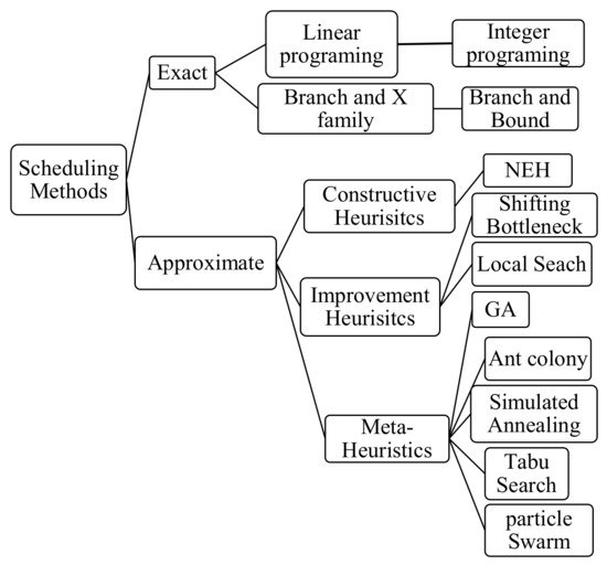
Figure 3. Classification of methods used to solve scheduling problems.

3.2.1. Exact Methods

Exact methods find the optimal solution once the problem has been solved ^[78]. Many exact methods are enumerative such that they explore so many solutions in a set number of iterations. This means that solving large-scale problems by using the exact method cannot be computationally feasible ^[80]. Due to the complexity of the real-world manufacturing systems, the recent papers dominantly focus applications of non-exact approaches. In our dataset, only 21% of the papers used exact method.

Some of the most applied exact methods to solve shop scheduling problem includes Linear and Dynamic Programming ^[81], mixed integer programming ^[82], and the Branch and X family (e.g., Branch and Bound algorithm, Branch and Price algorithm, Branch and Cut algorithm), etc., ^[83]. Integer Programming and Branch and Bound are particularly popular in the field of scheduling problems as we also observed in our dataset.

Integer programming and linear programming (LP) are simple and efficient optimization techniques which require the linear objective function and constraints. Linear programs can equivalently formulate dynamic programs ^[84]. The variables in integer programing are required to be integers and are sometimes constrained to binary.

Branch and bound (B&B) is also particularly popular in the field of scheduling problems. B&B (such as other Branch and X methods) decompose the problem into small disjoint subproblems to partition the solution space and generating a new lower bound for optimal cost ^[59]. It begins with an empty partial schedule and then unscheduled jobs are added to the top of the partial schedule, known as forward branching ^[59]. This eventually leads to multiple potential solutions. More information about the structure developed within a branch and bound algorithm can be found in Section 4.12.1.

3.2.2. Approximate Methods

Approximate methods do not necessarily find the optimal solution and may generate different results when solving the problem additional times ^[85]. Instead, approximate methods find good solutions in practical periods of time (unlike exact methods being time-expensive). Approximate methods are effective particularly in a case of NP-hard problem and large-scales problems ^[85].

Approximate methods include constructive heuristics, improvement heuristics, and meta-heuristics. Constructive and improvement heuristics differ in their starting search state (an empty versus an assumed pre-existing solution) while meta-heuristics utilize different high-level strategies to search ^[86].

Constructive heuristics form the solution from scratch and literally step by step, such that in each iteration, they choose the best available option ^[80]. The Nawaz, Enscore, Ham algorithm (NEH) is a constructive heuristic method observed multiple times in our dataset. This method sorts jobs in descending sums of processing times and then generates a job sequence by evaluating that sorted order of jobs through minimizing makespan ^[87].

Local search ^[28]^[88]^[89]^[90] and shifting bottleneck ^[91]^[92] are among Improvement heuristics which were repeatedly applied in our dataset.

Some of the more frequently occurring meta-heuristics from our dataset include genetic algorithms (GA), ant colony optimization algorithms (ACO), simulated annealing (SA), tabu search (TS), and particle swarm optimization algorithms (PSO).

Genetic algorithms (GA) imitate the evolutionary “survival of the fittest” behavior ^[78]. All possible solutions are represented as chromosomes, and chromosomes make up generations in which “survival of the fittest” is applied to eliminate suboptimal solutions and create a better next generation ^[78]. Eventually GA should reach a generation with a good or a close-to-optimal solution.

Ant colony optimization (ACO) method imitates the behavior of ants in their search for food using pheromones ^[86]. While randomly searching for food, artificial ants representing agents deposit pheromones along their path and subsequent ants choose paths with stronger pheromone concentrations ^[86], eventually leading to a good or a close-to-optimal solution.

Simulated annealing (SA) is a relatively simpler and older meta-heuristic. SA imitates the physical process of annealing, the cooling of a solid material and the subsequent arrangement of its particles, and uses the decrease of temperature in order to search for the optimal solution ^[86].

Tabu search (TS) extends the local search improvement method by incorporating other concepts to potentially find the close-to-optima such as best improvement (a method to move past local optima), tabu lists (limited memory to avoid cycles), and aspiration criteria (a work-around limited memory potentially locking out optimal solutions) in order to potentially find the close-to-optima ^[86].

Particle swarm optimization (PSO) imitates swarm intelligence by representing solutions as particles which then move around the state space toward theoretically better positions, until ideally converging to the global optima ^[33]^[40]. Particles move based on their own local neighborhood and based on the total findings within the swarm, reinforcing the idea of communication ^[93]^[94].

Algorithm 1 Solving a generic scheduling problem by an approximate method

1: Start with a random schedule or use a constructive method to generate a base schedule.
2: Calculate the performance measure
3: While a good solution (ideally, the optimal solution) has not been reached:
4: Perturb the schedule
5: Recalculate the performance measure

4. Theory and the Application of Different Types of Graphs

In this section, we discuss the theory of the most popular graph-based models utilized in different shop scheduling problems. It should be noted that general speaking there is a nested relation between the graph models and their equivalent matrix-based models. In some cases, matrix calculations are incorporated in the application of the graph-based model ^[95]. However, we kept the focus of this paper on the graph aspects.

Graphs model the relationships between objects rather than the objects themselves ^[96]. Two main elements of a graph are nodes and edges. Nodes (also known as vertices or points) represent the objects and edges (also known as links or arcs) show the relationship between the objects by connecting them. If a pair of nodes are connected by an edge, then these nodes are called as adjacent nodes. Edges can be directed or undirected, dictating the symmetry of the relationship between two nodes. Either edges or nodes in a graph can be weighted depending on the requirements of the system represented by the graph.

Let N and E be the set of nodes and edges in a given graph, then the graph can be denoted by G(N,E). A series of connected nodes create a path and if there is a path from node n ∊ N to m ∊ N, then m is reachable from n. Loop or cycle refers to a cyclic path such that all nodes on this cyclic path are reachable from themselves.

Figure 4 shows a comprehensive categorization over the most common graph-based models used in shop scheduling problems. The macro categorization is based on the existence of directed and undirected edges in different graph types. The third category entitled “Un/Directed” refers to those graphs which can potentially contain either directed or undirected edges, or those graphs which contains both directed and undirected at the same time.

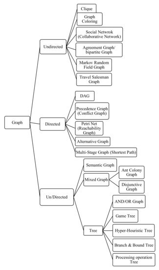
Figure 4. Categorization of different types of graphs.

In each subsection, after we introduce the concept, we will describe the application of the graph-based model to shop scheduling problems.

4.1. Clique

Clique is one of the fundamental concepts of graph theory ^[97]. To define clique, first we need to introduce a few concepts. Let C be a subgraph in an undirected graph G. Subgraph C is complete if each node within C is connected to every other node. C is maximal if C is a subset of G and is not contained in any other complete graph within G. Finally, $C$ is a clique if it is a complete maximal subgraph of G ^[98].

The maximum clique is the clique with the most nodes. The clique number, ω(G), dictates the number of nodes in the maximum clique within G ^[99].

Consider a random undirected graph in Figure 5. The maximum clique contains nodes {3,4,5,6} which is a 4-vertex clique. This clique is called a clique of size 4. Moreover, {3,4,5}, {3,5,6} are cliques of size 3 (3-vertix).

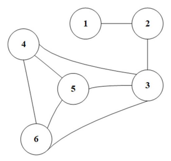
Figure 5. Random undirected graph.

The application of cliques to manufacturing/production related problems is mainly for partitioning ^[100] and simplifying classification ^[101]. We are particularly interested in its applications to shop scheduling problems where the concept of clique usually is coupled with graph coloring, agreement graph, and the disjunctive graph which are explained respectively in Section 4.2, Section 4.4, and Section 4.14.1.

4.2. Graph Coloring

Graph coloring assigns colors (or integer values) to nodes, and generally subject to the following constraint: no two adjacent nodes share the same color ^[97]. The colored graph is then optimized to reduce the number of colors applied ^[97].

This general definition of the graph coloring reveals the close connection between cliques and graph coloring, i.e., if G contains a clique of size k, then at least k colors are needed to color that clique. For instance, in Figure 5, at least four colors are needs for the clique of size 4. However, nodes 1 and 2 can have the same color of either nodes 4, 5, or, 6.

Color assignment can become more complex by encoding a set of colors rather than just a single color, known as multi-coloring ^[102]. With this, the sets of colors of two adjacent nodes must be disjoint ^[102].

Graph coloring is commonly used to model incompatible jobs which cannot be processed by the same machine ^[103]. Given an undirected graph G = (V,E), where V represents the set of jobs (nodes) and E is a set of edges between incompatible jobs ^[104]. Colors c are unique time units within the scheduling horizon and are assigned to a node if that corresponding job was processed at all during that time unit c ^[104]. The number of colors c are limited so as to not color each node uniquely, or equivalently processing each job one at a time. Another important concept is equitably c-colorable defined for a graph whose nodes can be divided into c independent sets ^[105].

Graph coloring can also be used for timetabling ^[106] and other potential constraints in shop scheduling problems. Graph coloring is conducive for exact and approximate methods to be applied ^[104].

4.3. Social Network (Collaborative Network)

Social networks, also known as a collaborative network, come from sociology and focus on how the interactions (edges) between actors (nodes) affect the collective, or the entire system ^[107]. Within this network, centrality measures are defined to focus on the most prominent actors (who are involved the most within the network, having the most incoming/outgoing edges) and their engagement in the network ^[107].

Recently, the social network has been utilized to model manufacturing systems as well. Social networks require a particular form of dataset as the input to be created. These datasets are summarized by the Affiliation matrix which is a symmetric Binary (Boolean) matrix where columns and rows shows the full list of all jobs, machines, and operations.

Reddy, Ratnam ^[107] represented a benchmark flexible job shop scheduling problem with 10 jobs and 6 machines using Affiliation atrix and collaborative network as in Figure 6. After modeling the problem, Reddy, Ratnam ^[107] identified key machines using centrality measures. This method creates descriptive statistics early on, helping to determine how sensitive the system may be when manipulating actors. After manipulation, metaheuristics can be re-run to conduct an accurate sensitivity analysis on key machines.

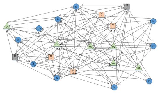
Figure 6. Collaborative network for the dataset 10 by 6 ^[107].

4.4. Agreement Graph and Bipartite Graph

An agreement graph is an undirect graph G = (V,E) where $V$ is the set of jobs (nodes) and E is a set of edges connecting a pair of agreeing jobs. Agreeing jobs are jobs that can be scheduled simultaneously on separate machines ^[108]. The agreement graph can be very useful when resources are non-sharable ^[108].

A bipartite graph, also known as a bigraph, is an undirected graph consisting of two disjoint independent sets of nodes, A and B, where V = A ∪ B Every edge connects a node in U to a node in V. Agreement graphs often are bipartite graphs since only pairs of agreeing jobs are graphed. Figure 7 shows a simple example of an agreement graph.

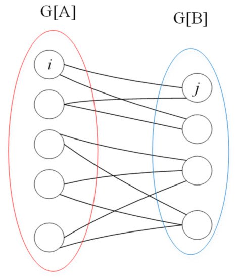
Figure 7. An agreement graph, G = (A ∪ B,E), that is also a bipartite graph in which agreeing jobs are connected by edges.

A tangible example of school exam planning can help the understanding of the concept of agreeing nodes (jobs) in the agreement graph of a shop scheduling problem ^[108]^[109]: suppose n exams need to be scheduled, equivalent to n jobs. Exams are scheduled to take place in m classrooms, equivalent to m machines, which can accommodate any exam. The objective is to minimize the examination period. The coinciding agreement graph for this situation would be an undirected graph, G = (V,E) such that V includes all of the jobs, J_i (exams), and E includes edges between jobs J_i and J_j if there are no students who take both exams (corresponding to those jobs) at the same time ^[108].

4.5. Markov Random Fields

Markov Random Fields (MRFs) are probabilistic graphical models and categorized as undirected graphs ^[110]. MRFs are used to model the existing correlation between the decision variables. Simply, MRF describes the dependency relationship of the variables. Nodes represent variables and edges represent the dependency between variables. That dependency can now be conditional according to the probabilities associated with each node.

In the shop scheduling context, the corresponding MRF model is defined as follows: Let (G,Φ) be a MRF where G = (N,A) is the graph structure (N is set of nodes and A is set of arcs) and Φ is parameters of the MRF. Nodes denote operations and an undirected arc between two nodes represent the correlation relationship between the two nodes.

Sun, Lin ^[110] used MRF to solve a real-world stochastic flexible job shop scheduling problem with the objective to minimize the expectation and variance of makespan. Unlike the traditional problem, in this stochastic scheduling problem the processing time of each operation is a stochastic value and not predefined. The concept of maximal clique is utilized to solve the stochastic problem which is modeled by MRF ^[110].

Despite the importance of stochastic nature of real-world manufacturing systems/processes, only one reference has been found (in our dataset) using MRF. We believe that shop scheduling field can clearly benefit from this graph-based approach in future. In addition to MRF, Bayesian network is another great probabilistic graph-based model that can potentially be utilized in shop scheduling problems.

4.6. Traveling Salesman Graph

The traveling salesman graph is a complete undirected graph with weighted edges where nodes represent cities and edges represent paths between cities such that weights of edge dictate distance ^[111]. Weights may also be assigned to nodes depending on the problem. A circuit that reaches each node once (and only once) is known as a tour and the length of a tour is the summation of weight of traversed edges. The objective of the problem associated with the traveling salesman graph is to find the optimal tour with the shortest length ^[111].

Traveling salesman graph is used to model the cyclic shop scheduling problem ^[112] which is a less common scheduling problem. Cyclic shop scheduling problem focuses on batches of products being produced over a fixed interval of time which is known as cycle time ^[66]^[112]. Cyclic scheduling problem looks to minimize cycle time ^[113].

Within a manufacturing context, the cyclic shop scheduling problem may have n jobs and m machines. A corresponding travel salesman graph can be defined for a kth machine in the cyclic problem by H_k(V,E,p,s) in which (V) represent jobs with weights corresponding to Operation Time (OP) and edges (E) represent the sequence of jobs with weights corresponding to Setup Times (ST). Then, the problem is formally defined, and the optimal schedule is equivalent to the optimal tour within a traveling salesman graph ^[112]. Figure 8 illustrates a sample of traveling salesman graph H_k.

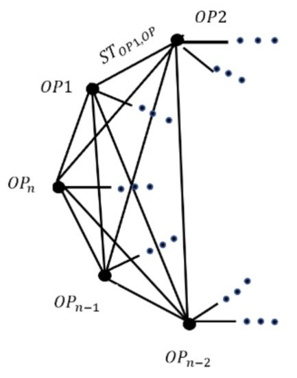
Figure 8. A partial graph H_k with parametric weights for nodes and edges.

4.7. Directed Acyclic Graph (DAG)

The Directed Acyclic graph (DAG) is the most important type of directed graph in the field of modeling the manufacturing systems. DAG can also explain some foundations for other types of directed graphs used in shop scheduling problems. Thus, we elaborated on some details of DAG and its mathematical background.

DAG is usually represented by the notation of G(N,E) where N is the set of nodes and E is the set of directed edges in G. Either nodes or edges can have weights. However, following the majority of references in our dataset, we considered weights on nodes in this paper.

Each node n has a set of predecessor and successor nodes which are connected to n through incoming edges and outgoing edges, respectively. A first node does not have any predecessors and a last node does not have any successors. Note that there might be multiple first and last nodes in a DAG. The length of the path to node n is calculated by the maximum of the summation of weights of nodes on the path from all first nodes to n ^[114]. The maximum of lengths of all paths from a first node to a last node is the length of the longest path, or the critical path which is an important measure in DAG calculation. The length of the longest path generally implies a critical performance measure in the corresponding system modeled by a DAG. It should be noted that the longest path can be defined only in directed graphs.

To find the length of the longest path, first the DAG should be topologically sorted, then, the length of the longest path to each node should be calculated using dynamic programing ^[22]. In the following subsection these two steps will be explained.

4.7.1. Topologically Sorting a DAG

To arrange nodes in a DAG, topological sorting is commonly done which converts nodes into linear order such that edges all point in one direction ^[115]. Multiple topological sorts can be defined for a DAG.

Kahn ^[116] proposed the most efficient algorithm known to find the topological sort in a DAG. A pseudo code of this Kahn’s algorithm is represented in Algorithm 2. Removing nodes from the dynamic set of Q (Step 4) is arbitrary. Different orders of removal result in a new, valid topological sort.

Algorithm 2 Topological Sort Algorithm

Output T, the set of nodes which are topologically sorted

1. Count the number of predecessors for all nodes using a counter Π
2. Insert all the first node with no predecessor in the dynamic set Q
3. While Q is not empty:
4. Remove a node from Q
5. Place the node in the topological set (T)
6. For all successors:
7. Decrement Π of the successor
8. If Π = 0
9. Insert the successor in Q

4.7.2. Calculating the Longest Path in a DAG

After topologically sorting the DAG, the dynamic programming algorithm finds the length of the longest path. Dynamic programing (also, known as dynamic optimization) is a popular mathematical optimization technique. It breaks down the problems into smaller sub-problems and try to find the optimal solution for the sub-problems to eventually solve the original problem. By applying dynamic programing methods, larger and more complex problems can be solved.

In DAG, an algorithm based on dynamic programming algorithm is proposed to find the longest path, L_max, by calculating the path of all nodes in topological order (Algorithm 3). In Algorithm 3, l_x denotes the length of the longest path from the first node to node x.

Note that T in Algorithm 3 is the output of Algorithm 2, and the data structure of T is predefined as a sorted set. Therefore, in step 2 of Algorithm 3, nodes are removed from T based on the topological order (the order of set T).

Algorithm 3: Finding the length of the longest path using Dynamic Programing Algorithm

Output l_n the length of the longest path to node n
L_max, the length of the longest path

1. For all nodes x on the topological sort (T):
2. Remove x from T
3.

l_{x} = \max_{n_{k} \in pred (x)} (l_{n_{k}}) + w_{x}

L_{m a x} = \max_{i \in L} (l_{i})

4.7.3. DAGs for Manufacturing Systems

If a DAG is used to model a manufacturing system, then it may be known as a task graph or precedence graph which will be explained in detail in Section 4.8 ^[117]. Within a manufacturing context, a manufacturing DAG’s (MDAG) can be defined where nodes represent operations with weights showing processing time. Also, edges represent the precedence of operations.

Ashour and Parker (1971) were among the pioneers applying a DAG/precedence graph to shop scheduling problem. They defined simple rules to model a system, i.e., horizontal edges represent the predefined route of a job, while vertical edges represent the schedule of a machine. Then, the length of the critical path is equivalent to the makespan, translating a manufacturing scheduling problem into a longest path search problem ^[118].

Figure 9 represents a job shop system and its topologically sorted version. Furthermore, Figure 10 depicts the flow shop system. In both examples, there are 4 jobs (J1 to J4) that should be processed by four machines (M1 to M4). The difference between the routings of flow shop and job shop system can be easily observed in these two figures. This confirms the powerfulness and simplicity of DAG as an appropriate graph-based models.

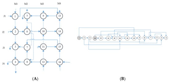
Figure 9. (A) Job shop DAG representation; (B) the topological sort of the DAG (Madraki & Judd, 2021).

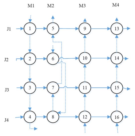
Figure 10. DAG representation of a flow shop systems.

4.8. Precedence Graph (Conflict Graph)

A precedence graph, also known as conflict graph, can be used to model a situation with constraints related to the concurrency of events. Two events that cannot be processed simultaneously are in conflict and therefore need a precedence relation to be defined ^[119]. The concept of a precedence graph has been visualized in several ways during its existence. In most references in our dataset, the precedence graphs are visualized as a DAG.

Birgin, Ferreira ^[120] proposed an efficient precedence graph in the flexible job shop scheduling problem. They used a similar approach to MDAG explained in Section 4.7.3. But they added a sequencing flexibility to the model. Also, they represented the precedence constraints of a single job as in Figure 11. This representation of precedence constraints seems to work well with industrial environments including the printing industry ^[88]^[121].

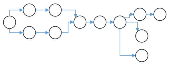
Figure 11. An example of precedence constrains of a single job in a flexible job shop system. An arbitrary DAG represents the precedence between operations of the job ^[119].

Although precedence graphs are mainly categorized as directed graphs, Tellache and Boudhar ^[122] defined an undirected graph as a precedence graph to model a flow shop scheduling problem. They discussed an interesting logical relevancy between their precedence graph and an associated agreement graph (which explained in Section 4.4) ^[108]. Instead of connecting agreeing jobs (nodes), this proposed precedence graph connects conflicting jobs ^[122]. Therefore, solving the FS problem with conflict graph is equivalent to solving FS problem with agreement graph.

4.9. Petri Net

Petri nets are directed bipartite graphs in which nodes are either classified as places (generally represented as circles) or transitions (generally represented as rectangles). Recalled from Section 4.4, in bipartite graphs, edges should connect nodes across the two disjoint groups. Edges pointing from a place to a transition are known as input places of a transition, and edges pointing from a transition to a place are known as output places of a transition. Places may acquire any number of tokens (depicts by dark filled circles as in Figure 12). If all input places connected to a transition have at least one token, then the transition is enabled.

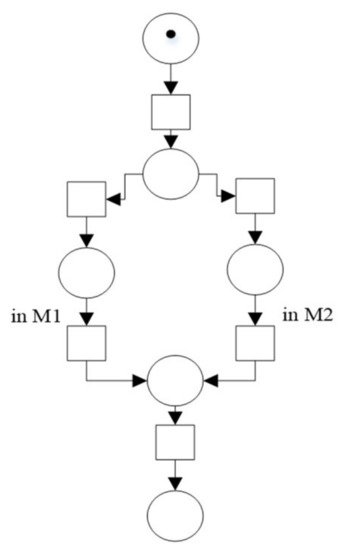
Figure 12. A petri net representing a manufacturing system with a job and 2 machine (M1 and M2) such that the job can be processed by either M1 or M2.

Once the transition is enabled and fires, it consumes the input places’ tokens and produces tokens in output places ^[51]. If more than one transitions are simultaneously enabled, then the transitions can fire in any order. Thus, firing of transitions and executing the petri nets are nondeterministic (unless an execution policy is defined). This means, systems with concurrent behavior, such as some manufacturing systems, can benefit from being modeled as a petri net.

Baccelli, Cohen ^[123] proposed an application of a particular type of petri net called as timed event graph to choice-free manufacturing systems. In timed event graphs, a node can have only one incoming and outgoing edge, while timing feature can be considered ^[124]^[125]. Moreover, timed event graph has been applied to model the job shop scheduling problem ^[126]^[127].

Figure 12 shows an example of a manufacturing system modeled by a petri net. This model includes six states denoted by places (circles), and six transitions which represent the changes between these states (rectangular). The states can be defined as follows: the process has not started, the process is being done by either machine 1 or machine 2, and the process is finished.

4.10. Alternative Graph

An alternative graph is a directed graph and denoted by G(N,F ∪ A) where N is the set of nodes and F ∪ A contains all edges. The edges in set F represents precedence relations and are usually visualized by the solid directed weighted edges. On the other hand, the edges in set A are alternative paths and visualized by doted/dashed edges ^[36]^[128]. Alternative edges can be weighted or not dictating whether swapping is allowed or not. In the context of shop scheduling problem, swapping refers to the ability for jobs to swap machines to avoid deadlock ^[37].

An alternative graph is a generalization of a disjunctive graph (described in Section 4.14.1) in which undirected edges represent the alternative path. Based on this, the disjunctive graph is categorized as a mixed graph, while the alternative graph is classified as a directed graph.

The alternative graph can be useful to model the scheduling problem with blocking situation (described in Table 1) ^[36]^[37]^[129]^[130]. In the corresponding alternative graph of a manufacturing system considering the blocking situation, nodes represent the operations. Edges in F showcase the precedence relation between consecutive operations, while edges in A showcase an alternative processing order for operations that cannot occur concurrently ^[37].

Figure 13 is an example for an alternative graph representing a partial manufacturing system with blocking situation. In this example, there are two operations i and j that cannot be done on the same time, i.e., these operations are processed by the same machine ^[36]. Also, σ_i and σ_j denote the operations associated with the blocking operations. Solid edges with weights show that i and j should be processed before σ_i and σ_j, respectively. Since i and j that cannot be done concurrently, dashed edges show alternative paths for them. Eventually, one of these alternatives will be selected.

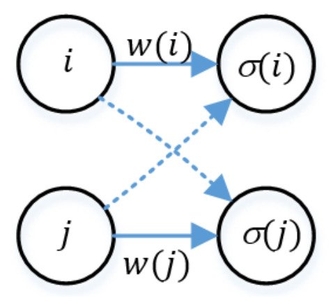
Figure 13. The alternative graph depicts a partial system with two operations i and j that cannot be processed at the same time.

4.11. Multi-Stage Graph

A multi-stage graph is a directed graph where nodes are grouped into stages and edges connect nodes from one stage to the next stage ^[131]. In a multi-stage graph, the goal is to find the shortest path from the first node to the last node, so, sometimes it is called as the shortest path problem.

The multi-stage graph has been used in several multi-stage shop scheduling problems such as multi-stage flow shop systems discussed in Section 2.2.4 ^[132]^[133], and classic open shop and job shop scheduling problems ^[24]. Within these applications, the combinations of the shop scheduling problems and the shortest path problem are studied using multi-stage graphs ^[133].

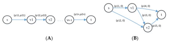
This so-called combination problem can be formally defined as follows: Let G = (V,E) be a directed graph with two distinguished vertices s,t ∊ V as a start and finish points which represents a manufacturing system with $m$ machines and $p$ jobs. Also, edges j ∊ E correspond to jobs J_j ∊ J, (j = 1, 2, …, p) and the weights on edges represent the processing time of jobs on the machines (p_1j, p_2j, …, p_mj). Then, the problem is to find a path from node s to t such that the appropriate schedule of jobs on machines yields the minimum makespan (or generally, with optimum performance measure) ^[24]. This is a combination of shop scheduling problem and the graph shortest path problem. It should be noted that the scheduling problem and the shortest path problem individually are two special cases of this so-called combination problem.

For instance, consider Figure 14A for a system with two machines and n jobs. Since in this figure, there is only one unique path from s to t, our problem is reduced to the two-machine shop scheduling problem. However, if we assumed that processing times on the second machine is zero, then, as shown in Figure 14B, then our problem is reduced to the shortest path problem ^[24].

Figure 14. Special cases of the combination problems using multi-stage graph. (A) a system with two machines. (B) the reduced problem to the shortest path problem.

4.12. Tree

A traditional tree is an undirected acyclic graph. However, a directed version of tree is also defined (it is called polytree). Nodes are connected by at most one edge. Adding any edge to a tree creates a cycle and deleting any edge in a tree makes the tree disconnected (having a node without any incoming or outgoing edge).

One of the applications of tree in the context of manufacturing systems is to build the critical tree based on the associated disjunctive graph (discussed in Section 4.14.1) representing a shop scheduling problem. A critical tree only considers the longest paths within a disjunctive graph, which allows for quick exploration of a potential schedule solution ^[134].

The rest of this section will discuss some of the most common types of trees and their applications in the scheduling problem that we could find in our dataset.

4.12.1. Branch and Bound Algorithm/Tree

As explained in Section 3.2.1, the branch and bound algorithm utilizes forward branching which appends unscheduled jobs to the head of the partial schedule developed. Throughout this process, a B&B tree is generated ^[135]. Nodes represent potential solutions and are branched such that their tree level corresponds to the number of jobs scheduled in that node ^[135].

4.12.2. Hyper-Heuristic Tree

A hyper-heuristic tree is used to select appropriate heuristics method or generate a new heuristics method which yields better solutions in a given search problem such as shop scheduling problem ^[136]. Genetic programming, a technique for breeding better solutions for a given problem ^[137], often goes hand-in-hand with hyper-heuristics. Trees are utilized in genetic programming hyper-heuristics to represent potential solutions (solutions being heuristics, not optimal schedules) ^[137]. Those trees are manipulated at the subtree level with the intent of breeding better solutions ^[23].

The hyper-heuristic tree is also used to solve a classical job shop scheduling problem by proposing a heuristic which consists of linear orders of dispatching rules: a tree structure is used to show each dispatching rule ^[138].

4.12.3. AND-OR Graph

An AND-OR Graph is a directed tree which utilizes some basic logic, including conjunction (and) and disjunction (or). AND/OR graph can provide a simple and visual understanding of a system, while it helps us to avoid unnecessary enumerating every alternative route of a given job in a scheduling problem ^[139]^[140].

AND/OR trees are typically made for each job, so nodes represent operations and directed edges present the predetermined route of a given job ^[141]. Logic is implemented, dictating whether the subsequent paths are all required (conjunction, represented by AND node) or either path is required (disjunction, represented by OR node) ^[139]. There are other methods for implementing logic, such as manipulating edges, which are also satisfactory.

One of the particular applications of AND-OR tree is to those problems where the shop scheduling problem is in a dynamic environment with alternative routes, such as flexible job shop ^[142], or with some kind of joining final assembly operation, such as flexible assembly job shop scheduling problem ^[139]. In such systems, each final product may be assembled from several subassemblies, and each subassembly may be assembled from several types of parts. Each part might go through linear or nonlinear process plans with operations on machines, as shown in an example in Figure 15.

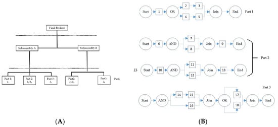
Figure 15. (A) An example of a flexible assembly job shop scheduling problem with three parts, two subassemblies. (B) AND/OR graph of machine operations of parts with alternative process plans ^[139].

4.12.4. Game Tree

Game theory and game trees are constructed based on the relationship between decision makers/players ^[143]. A game tree represents the decisions of players by assigning layers of a game tree to each player. Within that layer, nodes represent the different positions a player can choose from ^[144]. Directed or undirected edges represent moves a player can do. These edges connect nodes from a lower layer to a node in a higher layer which indicates that the choice of one player affects the choice of the next players since players make decision sequentially ^[144]. A game tree which includes every possible position and move is seen as complete.

The game tree is an efficient tool to model multiple objectives optimization problems such as shop scheduling problems since it can handle the competition and conflicts between the objectives ^[143].

In this application, objectives can be considered as players. Each objective (player) makes decision/ selects a feasible schedule based on its individual goal (e.g., minimizing makespan, minimizing total workload). Then, using dynamic game theory, the equilibrium solutions are considered as the optimal results of the multi-objective scheduling problem ^[143].

4.12.5. Processing Operation Tree

The integrated scheduling problem is defined when processing and assembly are performed simultaneously. This problem could be considered as a subset of the traditional job-shop scheduling problem. This problem produces a processing operation tree, also known as a tree-structured product-integrated scheduling, which is a directed tree where nodes represent operations and directed edges represent dependent relationships between the operations ^[145]. A processing operation tree is made for each job, like AND/OR graphs.

Figure 16 showcases a sample for a processing operation tree for a single job j that should be processed by 3 machines (M1, M2, and M3), through 15 operations (O1 to O15) ^[145].

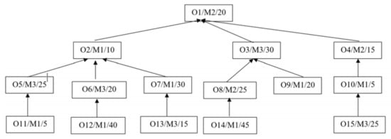
Figure 16. An example of a processing operation tree ^[145].

4.13. Semantic Graph

A semantic graph is a practical graph database and can be either directed or undirected. In a semantic graph, concepts and their relationships are represented by nodes and edges, respectively ^[146]. Unlike an ordinary graph in which edges can only represent the precedence relationships with possible quantitative weights, the edges in a semantic graph can also be assigned with semantic relations.

The distinguish advantage of a semantic graph is the ability to express qualitative and conceptual relationships compared to quantitative relationships. Semantic relations are encoded through a triple which refers to three entities relating to subject-predicate-object. Figure 17 shows an example for a triple.

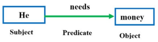
Figure 17. An example for a triple: ‘He needs money’.

Due to the special features of the semantic graph, it can integrate the entire lifecycle data of the system, and efficiently model many conceptual relationships that do exist in manufacturing systems beyond those represented numerically ^[146]. Examples of these relationships include stock constraints, sales orders, and other lifecycle data ^[146].

4.14. A Mixed Graph

Graphs which can contain both directed and undirected edges at the same timed are known as mixed graphs and they have some applications in different manufacturing systems. Disjunctive graphs and ant colony graphs are the most common mixed graphs to represent the shop scheduling problems. In this section, we will discuss these two models.

4.14.1. Disjunctive Graph

Disjunctive graph is one of the most used graph-based models in the field of shop scheduling. It was first proposed by Roy and Sussman, 1964 ^[81]. Disjunctive graphs can be compared to DAG when they are used to model a manufacturing system. Unlike DAG, in a disjunctive graph, the set of edges are represented by the union of two subsets of directed and undirected edges G = (V,C ∪ D) ^[147]. The operations are represented by nodes (V), and the route and the schedule are represented by the set of directed edges (C) and undirected edges (D), respectively. This means that the edges in C connect the sequential operations of each job. However, the undirected edges (D) between the operations show unspecified order of operations on a machine.

This ordering of all operations processed on each machine should be determined to find a good (ideally the optimal) schedule for the system. This can be done by using the concept of a clique. If all dashed edges are oriented such that each clique associated to a machine becomes acyclic then a feasible schedule is achieved. Thus, a schedule is feasible if and only if it can be represented by a directed acyclic disjunctive graph. Once the schedule is deemed feasible, the longest path from the oriented graph will compute makespan, the objective to be minimized.

Figure 18 illustrates a simple example of disjunctive graph representing a job shop system with 3 jobs (J0, J1, J2) and 3 machines (M0, M1, M2). Nodes $s$ and $t$ are dummy operations (nodes) showing the star and the end of the process. The rest of the nodes represent the operations, and the label of each node consists of two items: the machine which processes the operation and the operation time. By considering the dashed edges, a feasible schedule is determined where the length of the longest path (bold edges) is the makespan, i.e., 0 + 4 + 4 + 2 + 2 + 2 = 12.

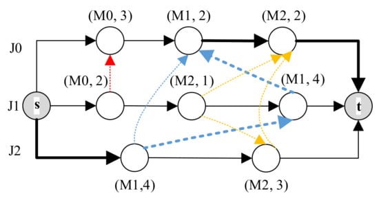
Figure 18. An example for a disjunctive graph representing a job shop system.

4.14.2. Ant Colony Graph

Ant colony graph or ants’ moving disjunctive graph ^[148] utilize the concept of disjunctive graphs to implement the ant colony optimization algorithm (detailed in Section 3.2.2) in shop scheduling problems.

In addition to all the same characteristics of a disjunctive graph, Ant colony graph include ants crawling from node to node across edges, leaving pheromones which increase the likelihood of taking that path again ^[148]^[149]^[150]. The ants resemble operations such that operations look for a machine to be processed on as quickly as possible just as ants look for food as quickly as possible when foraging ^[39]. The incorporation of dashed edges can be seen as an alternative path for searching ants ^[148]. The feasible solution is the directed path which visits every node, completing every operation ^[151].

References

Trudeau, R.J. Introduction to Graph. Theory; Courier Corporation: North Chelmsford, MA, USA, 2013.
Carlson, S.C. Königsberg Bridge Problem, in Encyclopedia Britannica. 2010. Available online: (accessed on 16 May 2021).
Mehrani, R.; Sharma, S. Behavior of water confined between hydrophobic surfaces with grafted segments. Colloid Interface Sci. Commun. 2021, 40, 100355.
Madraki, Y.; Oakley, A.; Le, A.N.; Colin, A.; Ovarlez, G.; Hormozi, S. Shear thickening in dense non-Brownian suspensions: Viscous to inertial transition. J. Rheol. 2020, 64, 227–238.
Riaz, F.; Ali, K.M. Applications of Graph Theory in Computer Science. In Proceedings of the 2011 Third International Conference on Computational Intelligence, Communication Systems and Networks, Bali, Indonesia, 26–28 July 2011; pp. 142–145.
Madraki, G.; Grasso, I.; Otala, J.; Liu, Y.; Matthews, J. Characterizing and Comparing COVID-19 Misinformation Across Languages, Countries and Platforms. arXiv 2020, arXiv:2010.06455.
Amato, F.; Castiglione, A.; De Santo, A.; Moscato, V.; Picariello, A.; Persia, F.; Sperlí, G. Recognizing human behaviours in online social networks. Comput. Secur. 2018, 74, 355–370.
Amato, F.; Moscato, V.; Picariello, A.; Sperli, G. Multimedia Social Network Modeling: A Proposal. In Proceedings of the 2016 IEEE Tenth International Conference on Semantic Computing (ICSC), Laguna Hills, CA, USA, 4–6 February 2016; pp. 448–453.
Otala, J.M.; Kurtic, G.; Grasso, I.; Liu, Y.; Matthews, J.; Madraki, G. 2021. Political Polarization and Platform Migration: A Study of Parler and Twitter Usage by United States of America Congress Members. In Companion Proceedings of the Web Conference 2021 (WWW ’21 Companion), April 19–23, 2021, Ljubljana, Slovenia; ACM: New York, NY, USA, 2021; p. 10.
La Gatta, V.; Moscato, V.; Postiglione, M.; Sperlì, G. CASTLE: Cluster-aided space transformation for local explanations. Expert Syst. Appl. 2021, 179, 115045.
Djakbarova, U.; Madraki, Y.; Chan, E.T.; Kural, C. Dynamic interplay between cell membrane tension and clathrin-mediated endocytosis. Biol. Cell 2021.
Mehrdad, S.; Mousavian, S.; Madraki, G.; Dvorkin, Y. Cyber-Physical Resilience of Electrical Power Systems Against Malicious Attacks: A Review. Curr. Sustain. Energy Rep. 2018, 5, 14–22.
Mousavian, S.; Conejo, A.J.; Sioshansi, R. Equilibria in investment and spot electricity markets: A conjectural-variations approach. Eur. J. Oper. Res. 2020, 281, 129–140.
Mousavian, S.; Erol-Kantarci, M.; Mouftah, H.T. Cyber-Security and Resiliency of Transportation and Power Systems in Smart Cities. In Transportation and Power Grid in Smart Cities; Wiley: Hoboken, NJ, USA, 2018; pp. 507–527.
Hosseini, S.; Ivanov, D. Bayesian networks for supply chain risk, resilience and ripple effect analysis: A literature review. Expert Syst. Appl. 2020, 161, 113649.
Salmani, Y.; Partovi, F.Y.; Banerjee, A. Customer-driven investment decisions in existing multiple sales channels: A downstream supply chain analysis. Int. J. Prod. Econ. 2018, 204, 44–58.
La Gatta, V.; Moscato, V.; Postiglione, M.; Sperli, G. An Epidemiological Neural Network Exploiting Dynamic Graph Structured Data Applied to the COVID-19 Outbreak. IEEE Trans. Big Data 2021, 7, 45–55.
Caggiano, A. Manufacturing System. In CIRP Encyclopedia of Production Engineering; Laperrière, L., Reinhart, G., Eds.; Springer: Berlin/Heidelberg, Germany, 2014; pp. 830–836.
Fan, K.; Zhai, Y.; Li, X.; Wang, M. Review and classification of hybrid shop scheduling. Prod. Eng. 2018, 12, 597–609.
Lamorgese, L.; Mannino, C. A Noncompact Formulation for Job-Shop Scheduling Problems in Traffic Management. Oper. Res. 2019, 67, 1586–1609.
Sobeyko, O.; Mönch, L. Heuristic approaches for scheduling jobs in large-scale flexible job shops. Comput. Oper. Res. 2016, 68, 97–109.
Madraki, G.; Bahalkeh, E.; Judd, R. Efficient Algorithm to Find Makespan under Perturbation in Operation Times. In Proceedings of the IIE Annual Conference, Institute of Industrial and Systems Engineers (IISE), Nashville, TN, USA, 30 May–2 June 2015; Institute of Industrial and Systems Engineers (IISE): Norcross, GA, USA, 2015.
Mei, Y.; Nguyen, S.; Xue, B.; Zhang, M. An Efficient Feature Selection Algorithm for Evolving Job Shop Scheduling Rules With Genetic Programming. IEEE Trans. Emerg. Top. Comput. Intell. 2017, 1, 339–353.
Nip, K.; Wang, Z.; Xing, W. A study on several combination problems of classic shop scheduling and shortest path. Theor. Comput. Sci. 2016, 654, 175–187.
Panwalkar, S.S.; Koulamas, C. The evolution of schematic representations of flow shop scheduling problems. J. Sched. 2018, 22, 379–391.
Zhang, J.; Ding, G.; Zou, Y.; Qin, S.; Fu, J. Review of job shop scheduling research and its new perspectives under Industry 4. J. Intell. Manuf. 2019, 30, 1809–1830.
Cao, Z.; Zhou, L.; Hu, B.; Lin, C. An Adaptive Scheduling Algorithm for Dynamic Jobs for Dealing with the Flexible Job Shop Scheduling Problem. Bus. Inf. Syst. Eng. 2019, 61, 299–309.
El-Desoky, I.; El-Shorbagy, M.A.; Nasr, S.M.; Hedaqy, Z.M.; Mousa, A.A. A hybrid genetic algorithm for job shop scheduling problems. Int. J. Adv. Eng. Technol. Comput. Sci. 2016, 3, 6–17.
Pinedo, M. Planning and Scheduling in Manufacturing and Services; Springer: Berlin/Heidelberg, Germany, 2005.
Clewett, A.J.; Baker, K.R. Introduction to Sequencing and Scheduling. Oper. Res. Q. 1977, 28, 352.
Wan, G.; Yen, B.P.-C. Tabu search for single machine scheduling with distinct due windows and weighted earliness/tardiness penalties. Eur. J. Oper. Res. 2002, 142, 271–281.
Guan, L.; Li, J.; Li, W.; Lichen, J. Improved approximation algorithms for the combination problem of parallel machine scheduling and path. J. Comb. Optim. 2019, 38, 689–697.
Behnamian, J. Graph colouring-based algorithm to parallel jobs scheduling on parallel factories. Int. J. Comput. Integr. Manuf. 2015, 29, 622–635.
Zabihzadeh, S.S.; Rezaeian, J. Two meta-heuristic algorithms for flexible flow shop scheduling problem with robotic transportation and release time. Appl. Soft Comput. 2016, 40, 319–330.
Mati, Y.; Dauzère-Pérès, S.; Lahlou, C. A general approach for optimizing regular criteria in the job-shop scheduling problem. Eur. J. Oper. Res. 2011, 212, 33–42.
Dabah, A.; Bendjoudi, A.; AitZai, A.; Taboudjemat, N.N. Efficient parallel tabu search for the blocking job shop scheduling problem. Soft Comput. 2019, 23, 13283–13295.
Pranzo, M.; Pacciarelli, D. An iterated greedy metaheuristic for the blocking job shop scheduling problem. J. Heuristics 2015, 22, 587–611.
Lange, J.; Werner, F. Approaches to modeling train scheduling problems as job-shop problems with blocking constraints. J. Sched. 2017, 21, 191–207.
Chaouch, I.; Driss, O.B.; Ghedira, K. A novel dynamic assignment rule for the distributed job shop scheduling problem using a hybrid ant-based algorithm. Appl. Intell. 2019, 49, 1903–1924.
AitZai, A.; Benmedjdoub, B.; Boudhar, M. Branch-and-bound and PSO algorithms for no-wait job shop scheduling. J. Intell. Manuf. 2014, 27, 679–688.
El Khoukhi, F.; Boukachour, J.; Alaoui, A.E.H. The “Dual-Ants Colony”: A novel hybrid approach for the flexible job shop scheduling problem with preventive maintenance. Comput. Ind. Eng. 2017, 106, 236–255.
Xie, J.; Gao, L.; Peng, K.; Li, X.; Li, H. Review on flexible job shop scheduling. IET Collab. Intell. Manuf. 2019, 1, 67–77.
Wu, J.; Wu, G.D.; Wang, J.J. Flexible Job-Shop Scheduling Problem Based on Hybrid ACO Algorithm. Int. J. Simul. Model. 2017, 16, 497–505.
Chen, J.C.; Wu, C.-C.; Chen, C.-W.; Chen, K.-H. Flexible job shop scheduling with parallel machines using Genetic Algorithm and Grouping Genetic Algorithm. Expert Syst. Appl. 2012, 39, 10016–10021.
Brucker, P.; Schlie, R. Job-shop scheduling with multi-purpose machines. Comput. 1990, 45, 369–375.
Dauzère-Pérès, S.; Paulli, J. An integrated approach for modeling and solving the general multiprocessor job-shop scheduling problem using tabu search. Ann. Oper. Res. 1997, 70, 281–306.
Zhao, B.; Gao, J.; Chen, K.; Guo, K. Two-generation Pareto ant colony algorithm for multi-objective job shop scheduling problem with alternative process plans and unrelated parallel machines. J. Intell. Manuf. 2018, 29, 93–108.
Prakash, A.; Chan, F.T.; Deshmukh, S. FMS scheduling with knowledge based genetic algorithm approach. Expert Syst. Appl. 2011, 38, 3161–3171.
Chan, F.T.S.; Chan, H.K. A comprehensive survey and future trend of simulation study on FMS scheduling. J. Intell. Manuf. 2004, 15, 87–102.
Błażewicz, J.; Ecker, K.H.; Pesch, E.; Schmidt, G.; Węglarz, J. Scheduling in Flexible Manufacturing Systems. In Scheduling Computer and Manufacturing Processes; Springer Science and Business Media LLC: Berlin/Heidelberg, Germany, 1996; pp. 369–421.
Baruwa, O.T.; Piera, M.A. A coloured Petri net-based hybrid heuristic search approach to simultaneous scheduling of machines and automated guided vehicles. Int. J. Prod. Res. 2016, 54, 4773–4792.
Gupta, J.N.; Stafford, E.F. Flowshop scheduling research after five decades. Eur. J. Oper. Res. 2006, 169, 699–711.
Ravindran, D.; Selvakumar, S.; Sivaraman, R.; Haq, A.N. Flow shop scheduling with multiple objective of minimizing makespan and total flow time. Int. J. Adv. Manuf. Technol. 2004, 25, 1007–1012.
Belabid, J.; Aqil, S.; Allali, K. Solving Permutation Flow Shop Scheduling Problem with Sequence-Independent Setup Time. J. Appl. Math. 2020, 2020, 1–11.
Motlagh, M.M.; Azimi, P.; Amiri, M.; Madraki, G. An efficient simulation optimization methodology to solve a multi-objective problem in unreliable unbalanced production lines. Expert Syst. Appl. 2019, 138, 112836.
Dallery, Y.; Gershwin, S. Manufacturing flow line systems: A review of models and analytical results. Queueing Syst. 1992, 12, 3–94.
Lee, C.-Y.; Cheng, T.C.E.; Lin, B.M.T. Minimizing the Makespan in the 3-Machine Assembly-Type Flowshop Scheduling Problem. Manag. Sci. 1993, 39, 616–625.
Wang, S.-Y.; Wang, L. An Estimation of Distribution Algorithm-Based Memetic Algorithm for the Distributed Assembly Permutation Flow-Shop Scheduling Problem. IEEE Trans. Syst. Man Cybern. Syst. 2016, 46, 139–149.
Gmys, J.; Mezmaz, M.; Melab, N.; Tuyttens, D. A computationally efficient Branch-and-Bound algorithm for the permutation flow-shop scheduling problem. Eur. J. Oper. Res. 2020, 284, 814–833.
Qian, B.; Li, Z.-C.; Hu, R. A copula-based hybrid estimation of distribution algorithm for m-machine reentrant permutation flow-shop scheduling problem. Appl. Soft Comput. 2017, 61, 921–934.
Ashrafi, M.; Davoudpour, H.; Abbassi, M. Investigating the efficiency of GRASP for the SDST HFS with controllable processing times and assignable due dates. In Handbook of Research on Novel Soft Computing Intelligent Algorithms: Theory and Practical Applications; IGI Global: Hershey, PA, USA, 2014; pp. 538–567.
Lee, T.-S.; Loong, Y.-T. A review of scheduling problem and resolution methods in flexible flow shop. Int. J. Ind. Eng. Comput. 2019, 10, 67–88.
Dorndorf, U.; Pesch, E. Solving the open shop scheduling problem. J. Sched. 2001, 4, 157–174.
Tellache, N.E.H.; Boudhar, M.; Yalaoui, F. Two-machine open shop problem with agreement graph. Theor. Comput. Sci. 2019, 796, 154–168.
Tellache, N.E.H.; Boudhar, M. Open shop scheduling problems with conflict graphs. Discret. Appl. Math. 2017, 227, 103–120.
Pempera, J.; Smutnicki, C. Open shop cyclic scheduling. Eur. J. Oper. Res. 2018, 269, 773–781.
Shakhlevich, N.V.; Sotskov, Y.N.; Werner, F. Complexity of mixed shop scheduling problems: A survey. Eur. J. Oper. Res. 2000, 120, 343–351.
Wang, M.; Zhong, R.Y.; Dai, Q.; Huang, G.Q. A MPN-based scheduling model for IoT-enabled hybrid flow shop manufacturing. Adv. Eng. Inf. 2016, 30, 728–736.
Pasupuleti, V. Scheduling in Cellular Manufacturing Systems. Iberoam. J. Ind. Eng. 2012, 4, 231–243.
Zeng, C.; Tang, J.; Yan, C. Job-shop cell-scheduling problem with inter-cell moves and automated guided vehicles. J. Intell. Manuf. 2015, 26, 845–859.
Neufeld, J.S.; Gupta, J.N.; Buscher, U. A comprehensive review of flowshop group scheduling literature. Comput. Oper. Res. 2016, 70, 56–74.
Yang, Y.; Chen, Y.; Long, C. Flexible robotic manufacturing cell scheduling problem with multiple robots. Int. J. Prod. Res. 2016, 54, 6768–6781.
Liu, C.; Wang, J.; Leung, J.Y.-T.; Li, K. Solving cell formation and task scheduling in cellular manufacturing system by discrete bacteria foraging algorithm. Int. J. Prod. Res. 2016, 54, 923–944.
Pinedo, M.; Hadavi, K. Scheduling: Theory, Algorithms and Systems Development. In Proceedings of the Operations Research Proceedings 1991; Springer Science and Business Media LLC: Berlin/Heidelberg, Germany, 1992; pp. 35–42.
Chen, B.; Potts, C.N.; Woeginger, G.J. A Review of Machine Scheduling: Complexity, Algorithms and Approximability. Handb. Comb. Optim. 1998, 1493–1641.
Stoop, P.P.; Wiers, V.C. The complexity of scheduling in practice. Int. J. Oper. Prod. Manag. 1996, 16, 37–53.
Lin, L.; Gen, M.; Liang, Y.; Ohno, K. A Hybrid EA for Reactive Flexible Job-shop Scheduling. Procedia Comput. Sci. 2012, 12, 110–115.
Amjad, M.K.; Butt, S.I.; Kousar, R.; Ahmad, R.; Agha, M.H.; Faping, Z.; Anjum, N.; Asgher, U. Recent Research Trends in Genetic Algorithm Based Flexible Job Shop Scheduling Problems. Math. Probl. Eng. 2018, 2018, 1–32.
Mokotoff, E. Parallel machine scheduling problems: A survey. Asia Pacif. J. Oper. Res. 2001, 18, 193.
Martí, R.; Reinelt, G. The Linear Ordering Problem: Exact and Heuristic Methods in Combinatorial Optimization; Springer Science & Business Media: Berlin/Heidelberg, Germany, 2011; Volume 175.
Kemmoé, S.; Lamy, D.; Tchernev, N. A Job-shop with an Energy Threshold Issue Considering Operations with Consumption Peaks. IFAC PapersOnLine 2015, 48, 788–793.
Sawik, T. Mixed integer programming for scheduling flexible flow lines with limited intermediate buffers. Math. Comput. Model. 2000, 31, 39–52.
Jourdan, L.; Basseur, M.; Talbi, E.-G. Hybridizing exact methods and metaheuristics: A taxonomy. Eur. J. Oper. Res. 2009, 199, 620–629.
Büyüktahtakin, I.E. Dynamic Programming Via Linear Programming. Wiley Encyclop. Oper. Res. Manag. Sci. 2010.
Williamson, D.P.; Shmoys, D.B. The Design of Approximation Algorithms. Design Approxim. Algorith. 2009.
Bianchi, L.; Dorigo, M.; Gambardella, L.M.; Gutjahr, W.J. A survey on metaheuristics for stochastic combinatorial optimization. Nat. Comput. 2009, 8, 239–287.
Framinan, J.M.; Leisten, R.; Ruiz-Usano, R. Efficient heuristics for flowshop sequencing with the objectives of makespan and flowtime minimisation. Eur. J. Oper. Res. 2002, 141, 559–569.
Lunardi, W.T.; Birgin, E.G.; Ronconi, D.P.; Voos, H. Metaheuristics for the online printing shop scheduling problem. Eur. J. Oper. Res. 2020.
Afsar, H.; Lacomme, P.; Ren, L.; Prodhon, C.; Vigo, D. Resolution of a Job-Shop problem with transportation constraints: A master/slave approach. IFAC PapersOnLine 2016, 49, 898–903.
Mencía, R.; Sierra, M.R.; Mencía, C.; Varela, R. Memetic algorithms for the job shop scheduling problem with operators. Appl. Soft Comput. 2015, 34, 94–105.
Shi, F.; Zhao, S.; Meng, Y. Hybrid algorithm based on improved extended shifting bottleneck procedure and GA for assembly job shop scheduling problem. Int. J. Prod. Res. 2020, 58, 2604–2625.
Choo, W.M.; Wong, L.-P.; Khader, A.T. A modified bee colony optimization with local search approach for job shop scheduling problems relevant to bottleneck machines. Int. J. Adv. Soft Comput. Appl. 2016, 8, 52–78.
Abdel-Kader, R.F. An improved PSO algorithm with genetic and neighborhood-based diversity operators for the job shop scheduling problem. Appl. Artif. Intell. 2018, 32, 433–462.
Nasiri, M.M. A modified ABC algorithm for the stage shop scheduling problem. Appl. Soft Comput. 2015, 28, 81–89.
Bahalkeh, E.; Madraki, G.; Judd, R. Efficient system matrix calculation for manufacturing systems. In Proceedings of the IIE Annual Conference, Nashville, TN, USA, 30 May–2 June 2015; Institute of Industrial and Systems Engineers (IISE): Norcross, GA, USA, 2015.
Weise, J.; Benkhardt, S.; Mostaghim, S. A Survey on Graph-based Systems in Manufacturing Processes. In Proceedings of the 2018 IEEE Symposium Series on Computational Intelligence (SSCI), Bangalore, India, 18–21 November 2018; Institute of Electrical and Electronics Engineers (IEEE): Piscataway, NJ, USA, 2018; pp. 112–119.
Sotskov, Y.N. Mixed Graph Colorings: A Historical Review. Mathematics 2020, 8, 385.
Moon, J.W.; Moser, L. On cliques in graphs. Isr. J. Math. 1965, 3, 23–28.
Prosser, P. Exact Algorithms for Maximum Clique: A Computational Study. Algorithms 2012, 5, 545–587.
Mohabeddine, A.; Boudhar, M. New results in two identical machines scheduling with agreement graphs. Theor. Comput. Sci. 2019, 779, 37–46.
Even, G.; Halldórsson, M.M.; Kaplan, L.; Ron, D. Scheduling with conflicts: Online and offline algorithms. J. Sched. 2008, 12, 199–224.
Halldórsson, M.M.; Kortsarz, G. Multicoloring: Problems and Techniques. In Proceedings of the International Symposium on Mathematical Foundations of Computer Science, Prague, Czech Republic, 22–27 August 2004; Springer: Berlin/Heidelberg, Germany, 2004; Volume 3153, pp. 25–41.
Furmańczyk, H.; Kubale, M. Scheduling of unit-length jobs with cubic incompatibility graphs on three uniform machines. Discret. Appl. Math. 2018, 234, 210–217.
Thevenin, S.; Zufferey, N.; Potvin, J.-Y. Graph multi-coloring for a job scheduling application. Discret. Appl. Math. 2018, 234, 218–235.
Furmańczyk, H.; Kubale, M. The complexity of equitable vertex coloring of graphs. J. Appl. Comput. Sci. 2005, 13, 95–106.
Ganguli, R.; Roy, S. A study on course timetable scheduling using graph coloring approach. Int. J. Comput. Appl. Math. 2017, 12, 469–485.
Reddy, M.S.; Ratnam, C.; Agrawal, R.; Varela, M.; Sharma, I.; Manupati, V. Investigation of reconfiguration effect on makespan with social network method for flexible job shop scheduling problem. Comput. Ind. Eng. 2017, 110, 231–241.
Bendraouche, M.; Boudhar, M. Scheduling with agreements: New results. Int. J. Prod. Res. 2015, 54, 1–15.
Bendraouche, M.; Boudhar, M.; Oulamara, A. Scheduling: Agreement graph vs resource constraints. Eur. J. Oper. Res. 2015, 240, 355–360.
Sun, L.; Lin, L.; Li, H.; Gen, M. Cooperative Co-Evolution Algorithm with an MRF-Based Decomposition Strategy for Stochastic Flexible Job Shop Scheduling. Mathematics 2019, 7, 318.
Rosenkrantz, D.J.; Stearns, R.E.; Lewis, P.M. Approximate algorithms for the traveling salesperson problem. 15th Ann. Sympos. Switch. Automata Theory 1974.
Bożejko, W.; Uchroński, M.; Wodecki, M. Block approach to the cyclic flow shop scheduling. Comput. Ind. Eng. 2015, 81, 158–166.
Bożejko, W.; Gnatowski, A.; Pempera, J.; Wodecki, M. Parallel tabu search for the cyclic job shop scheduling problem. Comput. Ind. Eng. 2017, 113, 512–524.
Madraki, G.; Judd, R. Accelerating the calculation of makespan used in scheduling improvement heuristics. Comput. Oper. Res. 2021, 130, 105233.
González, M.A.; Vela, M.D.C.R.; Varela, R. Scatter search with path relinking for the flexible job shop scheduling problem. Eur. J. Oper. Res. 2015, 245, 35–45.
Kahn, A.B. Topological sorting of large networks. Commun. ACM 1962, 5, 558–562.
Selvakumar, S.; Murthy, C.S.R. Scheduling precedence constrained task graphs with non-negligible intertask communication onto multiprocessors. IEEE Trans. Parallel Distrib. Syst. 1994, 5, 328–336.
Katriel, I.; Michel, L.; Van Hentenryck, P. Maintaining Longest Paths Incrementally. Constraints 2005, 10, 159–183.
Chen, Y.; Goebel, R.; Lin, G.; Su, B.; Zhang, A. Open-shop scheduling for unit jobs under precedence constraints. Theor. Comput. Sci. 2020, 803, 144–151.
Birgin, E.; Ferreira, J.; Ronconi, D. List scheduling and beam search methods for the flexible job shop scheduling problem with sequencing flexibility. Eur. J. Oper. Res. 2015, 247, 421–440.
Lunardi, W.T.; Birgin, E.G.; Laborie, P.; Ronconi, D.P.; Voos, H. Mixed Integer linear programming and constraint programming models for the online printing shop scheduling problem. Comput. Oper. Res. 2020, 123, 105020.
Tellache, N.E.H.; Boudhar, M. Flow shop scheduling problem with conflict graphs. Ann. Oper. Res. 2017, 261, 339–363.
Leake, C.; Baccelli, F.; Cohen, G.; Olsder, G.J.; Quadrat, J.-P. Synchronization and Linearity: An Algebra for Discrete Event Systems. J. Oper. Res. Soc. 1994, 45, 118.
Lee, T.-E.; Park, S.-H. An Extended Event Graph With Negative Places and Tokens for Time Window Constraints. IEEE Trans. Autom. Sci. Eng. 2005, 2, 319–332.
Cohen, G.; Gaubert, S.; Quadrat, J.-P. Max-plus algebra and system theory: Where we are and where to go now. Annu. Rev. Control. 1999, 23, 207–219.
Zhou, M.; Venkatesh, K. Modeling, Simulation, and Control. of Flexible Manufacturing Systems; World Scientific Pub Co Pte Lt: Singapore, 1999.
Zhou, M.; Dicesare, F.; DesRochers, A. A hybrid methodology for synthesis of Petri net models for manufacturing systems. IEEE Trans. Robot. Autom. 1992, 8, 350–361.
Lusby, R.M.; Larsen, J.; Ehrgott, M.; Ryan, D. Railway track allocation: Models and methods. OR Spectr. 2011, 33, 843–883.
Dabah, A.; Bendjoudi, A.; AitZai, A.; El-Baz, D.; Taboudjemat, N.N. Hybrid multi-core CPU and GPU-based B&B approaches for the blocking job shop scheduling problem. J. Parallel Distrib. Comput. 2018, 117, 73–86.
Gholami, O.; Krasemann, J.T. A Heuristic Approach to Solving the Train Traffic Re-Scheduling Problem in Real Time. Algorithms 2018, 11, 55.
Corominas, A.; García-Villoria, A.; González, N.-A.; Pastor, R. A multistage graph-based procedure for solving a just-in-time flexible job-shop scheduling problem with machine and time-dependent processing costs. J. Oper. Res. Soc. 2018, 70, 620–633.
Wang, S.; Liu, M.; Chu, C. A branch-and-bound algorithm for two-stage no-wait hybrid flow-shop scheduling. Int. J. Prod. Res. 2014, 53, 1143–1167.
Nip, K.; Wang, Z.; Nobibon, F.T.; Leus, R. A combination of flow shop scheduling and the shortest path problem. J. Combin. Optim. 2015, 29, 36–52.
Bierwirth, C.; Kuhpfahl, J. Extended GRASP for the job shop scheduling problem with total weighted tardiness objective. Eur. J. Oper. Res. 2017, 261, 835–848.
Kim, H.-J.; Lee, J.-H. Three-machine flow shop scheduling with overlapping waiting time constraints. Comput. Oper. Res. 2019, 101, 93–102.
Zhang, F.; Mei, Y.; Nguyen, S.; Zhang, M. Evolving Scheduling Heuristics via Genetic Programming With Feature Selection in Dynamic Flexible Job-Shop Scheduling. IEEE Trans. Cybern. 2021, 51, 1797–1811.
Zhou, Y.; Yang, J.-J.; Zheng, L.-Y. Hyper-Heuristic Coevolution of Machine Assignment and Job Sequencing Rules for Multi-Objective Dynamic Flexible Job Shop Scheduling. IEEE Access 2018, 7, 68–88.
Hart, E.; Sim, K. A hyper-heuristic ensemble method for static job-shop scheduling. Evolut. Comput. 2016, 24, 609–635.
Zhang, S.; Wang, S. Flexible Assembly Job-Shop Scheduling With Sequence-Dependent Setup Times and Part Sharing in a Dynamic Environment: Constraint Programming Model, Mixed-Integer Programming Model, and Dispatching Rules. IEEE Trans. Eng. Manag. 2018, 65, 487–504.
Rossi, A.; Lanzetta, M. Integration of hybrid additive/subtractive manufacturing planning and scheduling by metaheuristics. Comput. Ind. Eng. 2020, 144, 106428.
Liu, Q.; Li, X.; Gao, L.; Li, Y. A Modified Genetic Algorithm With New Encoding and Decoding Methods for Integrated Process Planning and Scheduling Problem. IEEE Trans. Cybern. 2020, 1–10.
Zhang, S.; Wong, T.N. Flexible job-shop scheduling/rescheduling in dynamic environment: A hybrid MAS/ACO approach. Int. J. Prod. Res. 2016, 55, 3173–3196.
Zhang, Y.; Wang, J.; Liu, Y. Game theory based real-time multi-objective flexible job shop scheduling considering environmental impact. J. Clean. Prod. 2017, 167, 665–679.
Rivest, R.L. Game tree searching by min/max approximation. Artif. Intell. 1987, 34, 77–96.
Lei, Q.; Guo, W.; Song, Y. Integrated scheduling algorithm based on an operation relationship matrix table for tree-structured products. Int. J. Prod. Res. 2018, 56, 5437–5456.
Zhu, Z.; Zhou, X.; Shao, K. A novel approach based on Neo4j for multi-constrained flexible job shop scheduling problem. Comput. Ind. Eng. 2019, 130, 671–686.
Grimes, D.; Hebrard, E. Solving Variants of the Job Shop Scheduling Problem Through Conflict-Directed Search. INFORMS J. Comput. 2015, 27, 268–284.
Wang, L.; Cai, J.; Li, M.; Liu, Z. Flexible Job Shop Scheduling Problem Using an Improved Ant Colony Optimization. Sci. Program. 2017, 2017, 1–11.
Qin, W.; Zhuang, Z.; Liu, Y.; Tang, O. A two-stage ant colony algorithm for hybrid flow shop scheduling with lot sizing and calendar constraints in printed circuit board assembly. Comput. Ind. Eng. 2019, 138, 106115.
Ciro, G.C.; Dugardin, F.; Yalaoui, F.; Kelly, R. Open shop scheduling problem with a multi-skills resource constraint: A genetic algorithm and an ant colony optimisation approach. Int. J. Prod. Res. 2015, 54, 4854–4881.
Riahi, V.; Kazemi, M. A new hybrid ant colony algorithm for scheduling of no-wait flowshop. Oper. Res. 2016, 18, 55–74.

© Text is available under the terms and conditions of the Creative Commons Attribution (CC BY) license; additional terms may apply. By using this site, you agree to the Terms and Conditions and Privacy Policy.

Upload a video for this entry

Information

Subjects: Engineering, Industrial; Operations Research & Management Science; Industrial Relations & Labor

Contributors MDPI registered users' name will be linked to their SciProfiles pages. To register with us, please refer to https://encyclopedia.pub/register :

Golshan Madraki

Jacqueline Otala

View Times: 1.5K

Update Date: 25 May 2021

Table of Contents