1. Introduction

Since the beginning of the 1990s, diffusion tensor magnetic resonance imaging has been extensively used in the experimental setting to characterise myocardial architecture in both autopsied [21] and beating hearts [22]. Even though several independent groups have used this imaging technique for more than 20 years, there is still no consensus on the appearance of the myocardial microstructure, the way in which we quantify the orientation of the cells, nor on interpretations relative to physiology and pathology [7]. The main principle behind quantification of myocardial architecture is the measurement of cardiomyocyte orientation. The cardiomyocytes are elongated cells measuring approximately 100 by 20 by 20 microns, and the overall goal is to assess the orientation of their long axis, as this is the main direction of force transmission. Diffusion tensor imaging achieves this by quantifying the direction and magnitude of Brownian motion of water molecules, that is the spontaneous diffusion occurring in both viable and fixed tissues [15]. In short, the result is presented as a three-dimensional mathematical construct called a tensor, the dimensions of which reflect the likely pattern of diffusion, itself a validated surrogate of the myocyte orientation (Figure 1). Likewise, computed tomography describes the myocardial morphology by the use of a tensor, but in this case the tensor is calculated by variations in x-ray attenuation within the tissue, where the direction of least difference is deemed to represent the longitudinal course of the myocyte chains. Consequently, this is referred to as a “structure tensor” rather than a “diffusion tensor” [18,23]. 

In general, a tensor is described using its three orthogonal axes. These are called eigenvectors, which are designated as being primary (e1), secondary (e2), and tertiary (e3). A complete mathematical description of a tensor is beyond the scope of this paper, but the interested reader is advised to consult specific literature dedicated to this matter [24]. To avoid confusion, it is important to note that owing to the underlying mathematical principles of tensor calculation, the long axis of the cardiomyocytes corresponds with the primary eigenvector in the diffusion tensor. Whilst in the structure tensor, the tertiary eigenvector aligns with the cardiomyocytes’ long axes [25,26]. The subsequent mathematical determination of myocyte orientation is identical for the two techniques. It has been rightfully argued that the main drawback of diffusion tensor imaging is its inability to assess the anatomy directly, instead using the spontaneous diffusion of water as a surrogate measure of the myocyte orientation [27]. Conversely, computed tomography, together with high-resolution conventional magnetic resonance imaging, provides the opportunity to evaluate the myocardial architecture based on tracking of actual anatomical features or “structures” [17,18]. This is an obvious advantage of computed tomography, but diffusion tensor imaging also holds important advantages. First of all, it is the only technique that currently holds potential as a clinical tool [28], and secondly it is the only validated and widely used methodology for assessing the orientation of the myocardial aggregates [7,17,29,30]. 

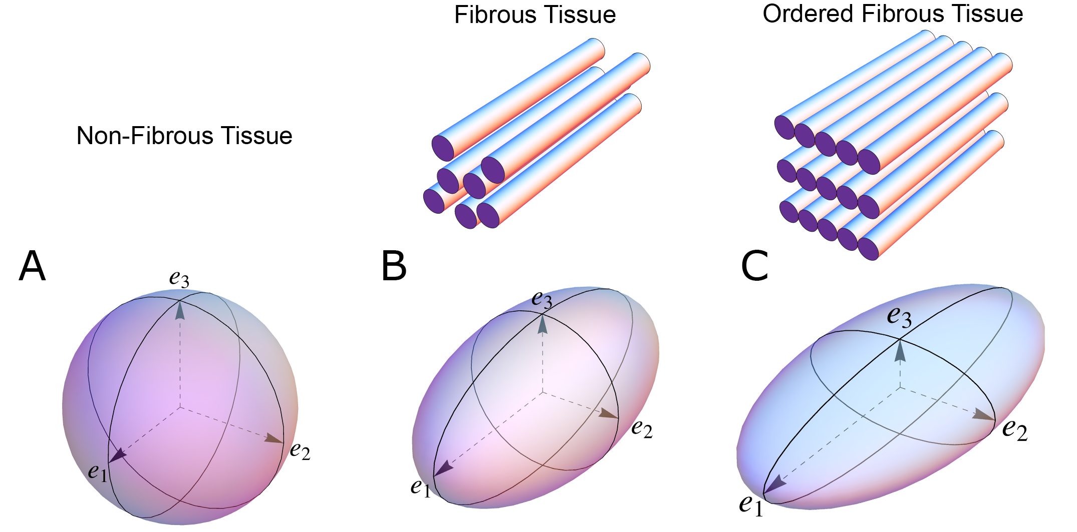
Figure 1. The shape of the diffusion tensor in different tissue environments. (A) Showing that all eigenvectors have equal magnitude in non-fibrous tissue resulting in a spherical shaped diffusion tensor. (B) Showing how, in fibrous tissue, the diffusion tensor takes on an ellipsoid shape when the magnitude of the primary eigenvector (e1) increases relative to the secondary eigenvector (e2) and tertiary eigenvector (e3). (C) In ordered tissue, the diffusion tensor can take on a flattened ellipsoid shape whereby the secondary eigenvector (e2) has a larger magnitude than the tertiary eigenvector (e3).

In an environment without cell membranes and other diffusion boundaries, the water molecules are equally likely to diffuse in all directions, thus the diffusion tensor assumes the shape of a sphere (Figure 1A). In biological tissues, whether within a cell or in the surrounding extracellular matrix, diffusion will be hindered mainly by the hydrophobic cell membranes. In tissues consisting of non-isotropic cells, such as in the brain or in muscles, the water diffuses most easily along the long axis of the cells. If the cells are grouped in common directional alignment, the tensor becomes an ellipsoid, with its long axis in the same direction as the common cellular long axis (Figure 1B). This configuration is typified by skeletal muscle, and by the long axonal tracts of the nervous system, particularly the spinal cord [31]. If the cells are also grouped into secondary substructures of reasonably regular shape, the signal from the extracellular water might cause differences in the magnitude of the secondary and tertiary eigenvectors. This is particularly the case when the cells are arranged so as to compartmentalise themselves in laminar fashion. As the myocytes in the laminar structure are aggregated tightly together, the water molecules are more likely to diffuse across this structure than through it. Thus, the secondary eigenvector will align with the plane of the laminar substructure, as this is the direction of greatest diffusion magnitude orthogonal to the primary eigenvector. Consequently, the diffusion tensor will assume a more flattened ellipsoid shape (Figure 1C). It is now well established that, in the myocardium, the primary eigenvector of the diffusion tensor follows the orientation of the chains of cardiomyocytes [21,32–35]. It has then been suggested that the secondary eigenvector follows the surface of the flattened groupings of cardiomyocytes, often described as myocardial sheets [32], laminae [9], sheetlets [36], lamellae [37], lamellar units [7,38] or aggregated units of cardiomyocytes [30]. This disagreement in nomenclature can be attributed to the current lack of a suitable three-dimensional anatomical description of these sub-structures. It is inherently difficult to assign a suitable name to a structure whose anatomical extent is unknown. Given our knowledge of their structural heterogeneity in size and thickness, we believe “myocardial aggregates”, as a name, currently provides the most suitable denomination. It was LeGrice and co-workers [39] who originally posited the existence of myocardial aggregates using electron microscopy. Computed tomography [8], confocal microscopy [19], ultrasound [40], and even photographically based methods [41], have also been used to evaluate the micro-anatomical features of the myocardial aggregates. None of these methods, however, can assess the aggregate normal vector, which we believe is key to calculating the precise orientation of the myocardial aggregates. To date, the normal of the myocardial aggregations has been assessed using diffusion tensor imaging [4], structure tensor calculation [42] and conventional histology [11]. Despite this, the most prominent approach is to assess myocardial aggregate orientation using the in-plane secondary eigenvector, which we claim is not founded in mathematical theory.

Many investigators are now exploring the remodelling of myocyte orientation in disease, with results now emerging characterising changes in hypertrophic and dilatated cardiomyopathies, and congenital malformations [16,26,43–45]. This has led to the desire to explore the prognostic and diagnostic potential of myocyte orientation analysis [28], thus knowledge of its technical limitations and methodological inconsistencies is paramount. 

2. Assessing Myocardial Architecture

2.1. Establishing Reference Points

In order to describe the orientation of the chains of cardiomyocytes, it is agreed that unique points of reference are needed. There is general agreement in the published literature that, in the first instance, the global orientation of the heart itself should be described using the left ventricular long axis. This is usually achieved by placing a line between the apex and the fibrous continuity between the leaflets of the aortic and mitral valves [39,45–47]. An alternative approach is to interpolate a line between the centres of the ventricular cavity in a series of short axis images [25,48–51]. The left ventricular long axis, along with two orthogonal radial vectors (e_R1 and e_R2), then provides the global geometric coordinate system for defining the position of the heart (Figure 2A). In some studies, these are the only points of reference used when assessing myocytic orientation [51–53].

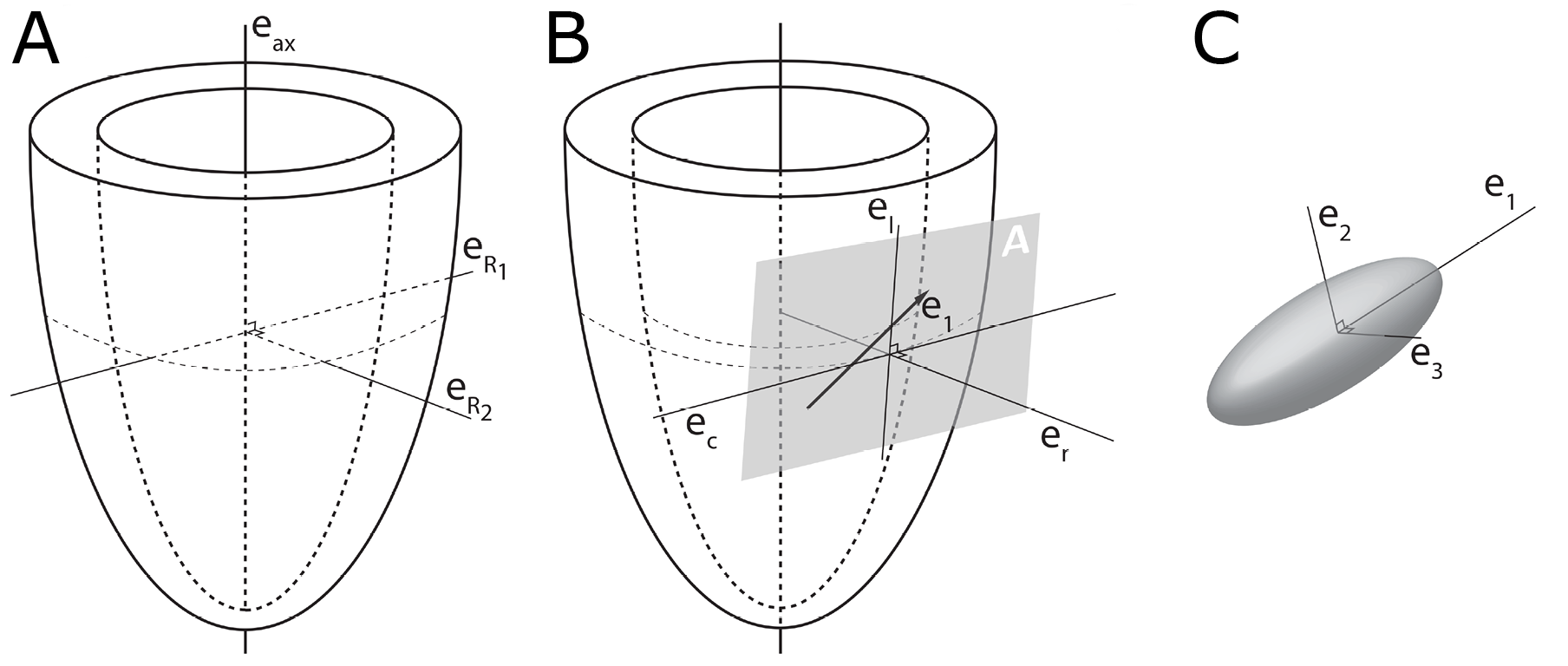
Figure 2. Establishment of the reference planes. (A) Illustrates the global geometric coordinate system defining the position of the left ventricle. It is defined by the orthonormal basis [eax→,eR1→,eR2→] where eax→ is the left ventricular long axis and eR1→ and eR2→ being orthogonal radial vectors, which are not used in the determination of myocyte orientations. (B) Subsequently, the local wall coordinate system is defined based on the orthonormal basis [er→,ec→,el→], where er→ is the local radial vector, i.e., the normal of the epicardial tangential plane A, el→ is the local longitudinal vector, i.e., the normal of the local horizontal plane, and lastly ec→ is the local circumferential vector. (C) Finally, the diffusion tensor is defined by a sub-local coordinate system based on the orthonormal bases [e1→,e2→,e3→], which are the three eigenvectors. Modified from [25].

2.2. The Helical Angle

In order to completely describe the orientation of a vector in a three-dimensional space, one needs to assess its orientation relative to two reference planes [58]. It is Streeter and his colleagues who are usually credited with introducing the notion of the helical angle (Figure 3B), which assesses myocyte orientation relative to the equatorial/horizontal plane of the ventricular cone [59,60]. However, this notion of change in myocyte angle relative to transmural position goes further back in time [61]. The idea that such angulation could be assessed relative to the horizontal plane was originally introduced by Feneis [62]. The notion was later endorsed by Hort [63] when the latter performed his extensive investigations of myocardial structure. Such helical angles are considered positive in the sub-endocardium, approximately zero in the mid-wall, and negative in the sub-epicardium. 

2.3. Transmural Orientation

Once the helical orientation of the cardiomyocytes is determined relative to the local horizontal plane of the left ventricle (α in Figure 3), it also becomes necessary to consider any change in transmural orientation relative to the epicardial tangential plane (Figure 3). Once these two angles are defined, one has established the precise orientation of the cardiomyocytes. Thus, it is the combination of the helical and transmural orientations that provides the complete anatomical description of the orientation of the cardiomyocyte chains [25]. The notion of transmural angulation (i.e., across the wall) was also investigated by Streeter and his colleagues, and consequently named by them: the angle of imbrication [75]. This term, however, has not survived the passage of time. A significant number of morphological studies, nonetheless, have explicitly denied the existence of populations of cardiomyocytes aggregated together with transmural orientation [10,34,36,51,66–68,76–78]. Evidence now confirms that transmural angulations do indeed exist [4,13,55,79], and it is suggested they play a key role in cardiac function [54,56,80]. The notion of mural antagonism and its functional significance [2,80] is yet to gain field-wide acclaim; this may be due, in part, to the historical dogma attached to the existence of transmurally arranged cardiomyocytes. 

2.4. Myocardial Aggregate Orientation 

Studies of the supporting fibrous matrix have shown that the cardiomyocytes are packed together in functional subunits [87]. This notion of packing led LeGrice and colleagues to propose that the ventricular walls are organised in anatomical aggregations of a laminar nature [9]. The extent of such myocardial aggregations and their role in both the compartmentalisation and deformation of the ventricular walls remain two of the most discussed controversies in cardiac morphology. These aggregations are of major importance as they facilitate the continuous rearrangement and deformation of the myocardium through the cardiac cycle [4,28]. Assessment of aggregate orientation (Figure 3) has been shown to be a reliable marker of cardiac disease [28], but the method of assessment is heavily disputed [25].

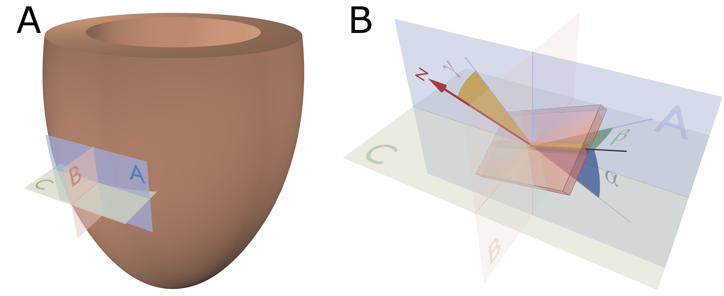
Figure 3. Reference planes and angle definitions. (A) showing a schematic of the left ventricle with the local orthogonal reference planes aligned with the epicardium. Plane A is parallel to the epicardial tangential plane, while the orthogonal plane B is parallel to the left ventricular long axis. Consequently, plane C is orthogonal to both planes A and B and is often referred to as the local “horizontal” plane. (B) Outlines our recommended angle definitions. The helical angle α is the angle between the primary eigenvector (black line) and plane C. The intrusion angle β is the angle between the primary eigenvector and plane A. Lastly, the aggregate angle is measured using the aggregate plane normal (N) assessed against the epicardial tangential plane A. The unit of aggregated cardiomyocytes is depicted as the yellow box, which is a schematic oversimplification.

2.5. Consequences of Projected Angles 

It is frequent to find studies where vectors of diffusion tensors have been projected onto reference planes prior to assessing their angulations [25]. If we accept the fact that not all cardiomyocytes are arranged in surface parallel fashion, or in other words that myocyte chains exhibit a transmural angle, we must also accept that projected angles are prone to bias or anatomically inaccurate results. Previously we assessed the consequences of projection when calculating helical, transmural, and aggregate angle [25]. The larger the transmural angulation, the more the corresponding projected helical angle deviates away from its true value. The transmural angulation of cardiomyocytes is particularly sensitive to projection, with the larger the helical angle, the greater the deviation of the projected transverse angle away from the true transmural angle. Also, the aggregate orientation is sensitive to projection, thus we generally recommend avoiding the use of projection.

This entry is adapted from the peer-reviewed paper 10.3390/jcdd7040047