The artificial neural network (ANN) used today is the product of the combined efforts of a number of researchers, including McCulloch et al. [1], who first developed the concept in 1943. The concept of the convolutional neural network (CNN), among the most widely used neural network structures in computer vision (CV) applications, was first introduced using LeNet-5 in a 1989 study by LeCun et al. [2]. Back then, however, due to the lack of computing power of the hardware, CNN was found to be ineffective in dealing with complex and sophisticated tasks, such as object recognition and detection. After quite a while, AlexNet [3] was first introduced at the ImageNet Large Scale Visual Recognition Challenge (ILSVRC) in 2012; it made an impressive debut because the model was able to effectively overcome the limitations of deep learning (DL), making the most of GPU computing. With its unparalleled performance, AlexNet ushered in a new era of DL in earnest [4]. DL has attracted significant attention from researchers thanks to its ability to allow the automatic extraction of valid feature vectors from image data. Performing this automatic extraction requires the tuning of the hyper-parameters of DL. Thus far, extensive research for improved performance has been performed on a wide range of hyper-parameters, such as network structures, weight initialization, activation functions, operators, and loss functions [5,6,7,8,9]. However, the application of DL requires technical expertise and understanding, while incurring a significant amount of engineering time. In attempts to address these issues, automated machine learning (AutoML) has recently garnered significant attention.

The AutoML process is divided into multiple steps, including data preparation, feature engineering, model generation, and model estimation [10]. The first step of AutoML, data preparation, is a process in which data are collected; factors that may negatively affect the learning process, e.g., noise, are removed to train a given model to perform the target tasks. The second step, feature engineering, extracts features from given data to be used in the model. At the same time, feature construction techniques to improve the representative ability of the model, as well as feature selection techniques used to avoid overfitting, are applied in parallel. Conventional feature engineering methods include SURF [11], SIFT [12], HOG [13], the Kalman filter [14], and the Gabor filter. Recently, CNN and recurrent neural network (RNN) applications have been used to extract high-level features. The third step, model generation, is performed to obtain optimum output based on the extracted features. Model generation can be further subdivided into search space, hyper-parameters, and architecture optimization. During this process, model optimization is performed in combination with the model estimation step.

If we simply think of the mechanism of a neural network, it is a graph composed of many operations, and it is a set of operations aimed at transforming from input data to expected output data. Such an expression can be represented by a directed acyclic graph (DAG) as Equation (1) [15]. where s^(t) indicates a state at t s^(t)∈S (is equal to the k^th node of the neural network), and s^(t−1) and o^(t) represent a previous state and its associated operation o^(t)∈O, respectively. O includes various series of operators such as convolution, deconvolution, skip-connection, pooling, and activation functions.

Neural architecture search space consists of a set of candidate operators and a restricted space in which the operators are placed. The operators of the candidate set depend on the task of the neural network. Most NAS research competes for performance through classification challenges in the CV field. In this case, convolution, dilated convolution [16], depth-wise convolution [17], etc., are widely used for candidate set. 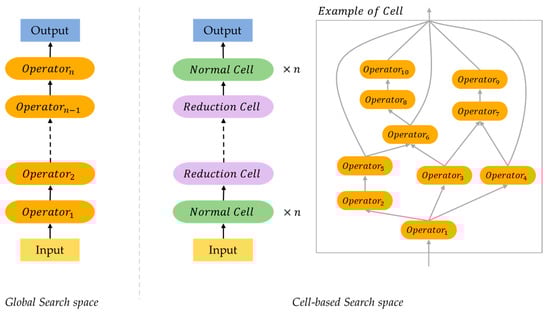Search Space has various methods such as Sequential LayerWise Operations [18,19], Hierarchical Brench Connection Operations [20], Global Search space, Cell-Based search space [21], and Memory bank representation [22]. This text will discuss the search space divided into global search space and cell-based search space. Figure 1 shows a simple example structure of both methods.

The global search space is equivalent to finding the series of operators O of the DAG. In other words, it is to determine the operator set with the best performance for a predefined number of nodes between the initial input and the final output. Searching the entire structure has several unavoidable disadvantages. Typically, most deep neural networks used in recent research consist of tens to hundreds of operators. If the global search method is applied to these networks, considerable GPU time will be required.

Cell-based search space is based on the fact that the latest and successful artificial neural network structures [23,24,25] consist of repetitions of cells (also known as modules, blocks, units). Typical examples of such cell structures are a residual cell of ResNet [23] and a dense cell of DenseNet [24]. Since the aforementioned neural network structures are flexible in controlling the number of cells, the size of the structure can be determined by optimizing it for a scenario.

NAS research using cell-based search space was introduced in NASNet [21]. NASNet is a structure in which a reduction cell and a normal cell are found through RNN and reinforcement learning, and the final architecture is determined by stacking them several times. In [21], the computational cost and performance was improved compared to the state-of-the-art alternatives (e.g., Inception v3 [26], ResNet [23], DenseNet [24], ShuffleNet [27], etc.).

As the search space is determined, we need a solution to search for the optimal neural architecture. To automate architecture optimization, traditional techniques up to the latest techniques are being studied. After architecture search, most NAS methods use grid search, random search, Bayesian Optimization, or gradient based optimization for hyperparameter optimization [10]. Table 1 compares the performance and efficiency of NAS algorithms using the CIFAR-10 and ImageNet dataset.

An evolutionary algorithm (EA) is a metaheuristic optimization algorithm inspired by evolutionary mechanisms in biology such as reproduction, mutation, and recombination. Specifically, an EA finds the optimal solution by repeating the steps of ‘evaluating the fitness of individual’, ‘selecting the individuals for reproduction’, and ‘crossover and mutation operation’. Because this algorithm does not have to assume fitness ideally, it can perform well in approximate solutions for many types of problem.

One of the most popular types of EA is the genetic algorithm (GA). The GA aims to transmit superior genetic information to the next generation by selecting competitive individuals from current generation. Genetic information for NAS includes information about neural network architecture, and each generation is accompanied by a training process to evaluate the performance of neural network architecture. This issue shows the limitation of the EA-based NAS method that requires significant GPU time. The schematic process of GA-based NAS can be summarized as Algorithm 1.

Algorithm 1 GA-based NAS Algorithm

1: Input: the number of generations T, the number of individuals in each generation N, the dataset D; 2: Initialization: generating the initial individuals randomly; 3: For 1,2,3, …, T do; 4: For 1,2,3, …, N do; 5: Evaluation: neural network architecture (individual) training for D_train; 6: Evaluate the performance of the neural network architecture for D_test; 7: end for 8: Selection: selecting the most suitable individuals for reproduction; 9: Crossover and Mutation: reproducing new individuals; 10: end for 11: Output: individuals in the last generation.

In the case of NAS based on the GA, it is important to optimize the structure of the neural network through its genetic representation. Rikhtegar et al. [28] utilized the genetic representation encoded as integers for the number of filters, the size of filters, interconnection between feature maps, and activation functions. Using this encoding method, it is possible to find optimal parameters of neural network architecture, but the number of layers is fixed and it is only possible to search for a pre-defined connection structure. Xie et al. [29] designed a genetic representation focusing on the connection structure of convolutional layers. Their encoding method expressed the validity of the connection between each convolutional layer as a fixed-length binary string. However, contrary to [28], multiscale information cannot be utilized because the number of filters and size of filters are fixed.

Reinforcement learning (RL), inspired by behavioral psychology, is a method of machine learning in which agents learn in a predefined environment to select actions that seek to maximize the reward obtainable in the current state. Zoph et al. [18] is one of the earliest applications of reinforcement learning for NAS. They argued that Recurrent Neural Network (RNN) can be used as a NAS controller based on the fact that the structure and connectivity of the neural network can be expressed as a variable-length string. The RNN-based controller has the strength to flexibly respond to the architecture structure. In addition, the overall process speed was increased by using the asynchronous parameter updates for the controller and the distributed training for the child network [30]. In the same year, Baker et al. [19] proposed a MetaQNN that combines two techniques with Q-learning.

In traditional reinforcement learning, the convergence speed is slow due to over-exploration, and there is a problem if there is convergence to the local minima due to over-exploitation [40]. Baker et al. applied facts that can overcome these two problems with an ε-greedy strategy [41] and experience replay [42]. Zhong et al. [31] also introduced BlockQNN using the Q-learning paradigm with ε-greedy exploration strategy. However, unlike [19], they adopted a cell-based search space, referring to the fact that superior hand-crafted networks such as GoogLeNet [43] and ResNet [23] have the same block stacked structure. In [31], BlockQNN demonstrated advantageous in computational cost and strong generalizability through experiments. Inspired by the concept of ‘weight inheritance’ in [44], Pham et al. introduced ENAS [32], which applies a parameter sharing strategy to child architecture. According to the experimental results of [32], a searching time less than 16 h was required with a single GPU (GTX 1080Ti) on CIFAR-10. This result means that the GPU time is reduced by more than 1000× compared to [18], and it shows considerable efficiency in terms of computational cost.

Since the EA and RL search strategies are based on a discrete neural network space, a lot of search time is required. To solve this problem, studies on how to apply gradient-descent optimization techniques by transforming the discrete neural network space into continuous and differentiable spaces have been published. In 2018, Shin et al. [45] published DAS that solved the NAS as a fully-differentiable-problem, further developing from studies [46,47,48] that partially utilized the continuous domain concept. However, DAS has a limitation of optimizing only specific parameters of an architecture. DARTS [33] published by Liu et al. in 2019 focused on learning the complex operation graph topologies inside the cell constituting the neural network architecture. The DARTS is not limited to a specific neural network architecture, and has been the basis for many studies [34,35,36,37,38] as it can search both CNN and RNN. Liang et al. [34] observed performance collapse as the number of epochs of DARTS increased, and found that this was a result of overfitting due to the number of skip-connections that increased with epochs. They solved the performance collapse problem through DARTS+ [34], which applied the ‘early stopping’ technique, based on the research results that important connections and significant changes were determined in the early phase of training [49,50,51]. Chu et al. proposed Fair-DARTS [35], which applied independence of each operation’s architectural weight to solve the performance collapse problem caused by skip-connection, and eliminated the unfair advantage. Chen et al. [36] proposed progressive DARTS (P-DARTS) to solve the depth gap of DARTS. The depth gap is a problem that occurs in cell-based search methods, and is a performance collapse problem that occurs when different networks operate in the search phase and the evaluation phase. To solve the depth gap problem of DARTS, where the number of cells in the search phase and estimation phase are 8 and 20, respectively, P-DARTS reduced the difference from the estimation phase by gradually increasing the number of cells in the search phase. PC-DARTS [39] proposed by Xu et al. improved memory efficiency through random sampling for operation search and used a larger batch size for higher stability.

In addition to search space and search strategy, evaluation strategies are very important to improve NAS performance. An efficient NAS performance evaluation strategy can speed up the entire neural architecture search process while reducing the cost of computing resources. The simplest and most popular method, early-stopping [34,52,53,54] was widely used, but search results mostly showed simple and shallow layers. In general, these networks can be fast in terms of speed, but often have poor performance. The technique of parameter sharing is used to accelerate the process of NAS. For example, ENAS [32] constructs a large computational graph to perform a considerable amount of computation so that each subgraph represents a neural architecture and all architectures share parameters. In that way, this method improves the efficiency of NAS by avoiding training sub-models from scratch to convergence. Network morphism based algorithms [55,56] can also inherit the parameters of previous architectures, and single-path NAS [57] uses a single-path over parameterized ConvNet to encode all architectural decisions with a shared convolutional kernel. Another strategy is to use a proxy dataset. This method [58] is used by most existing NAS algorithms and can save computational cost by training and evaluating intermediate neural architectures on a small proxy dataset with limited training epochs. However, it is difficult to expect an architecture search with good performance with this coarse evaluation method.

Recently, various Evaluation Strategies are being studied to overcome the disadvantages of NAS. ReNAS [59] tries to predict the performance ranking of the searched architecture instead of calculating the accuracy as another strategy to accelerate the search process. In 2021, CTNAS [60] completely transforms the evaluation task into a contrastive learning problem. By proposing a method, an attempt is made to calculate the probability that the performance of the candidate architecture is better than the baseline. Most recently in 2022, ERNAS [61] proposes an end-to-end neural architecture search approach and a gradient descent search strategy to find candidates with better performance in latent space to efficiently find better neural structures.