1. Introduction

Euclidean graph-based image analysis is a special technique particularly suited for the identification and processing of curvilinear features in digital images ^[1]. The analysis of line-shaped features in images is involved in several fields including, among others, civil engineering (e.g., surface cracks on concrete ^[2] and stainless steel ^[3]), biology and medicine (e.g., blood vessel analysis ^[4] and neuron tracing ^[5]) and general image analysis ^[6][7]. Particularly, in civil engineering, the detection and measurement of structural cracks is of primary importance in the structural assessment of built structures, with an ever growing interest for automated concrete crack detection and analysis methods because of the progressive ageing of civil constructions, especially in the Western world (with more than 50% of the residential building stock built before 1969 in several European countries ^[1]). The typical process of curvilinear feature analysis in digital images is subdivided into a first detection phase, where the possible objects of interests are identified through a specific image segmentation method, and a subsequent post-detection phase, where the object recognized in the binarized image is refined, selected and analyzed. Euclidean graphs are an ideal data structure for the description of curvilinear features recognized in a binarized image, capturing the essentials of the object paths and ensuring an effective computational availability of its main features for the following analysis process.

2. Euclidean Graphs

A Euclidean graph (EG) is a weighted graph where each vertex corresponds to a point in a Euclidean space (Figure 1) and each edge weight is proportional to the Euclidean distance between its two endpoints. Like ordinary graphs, EGs can consist of several subgraphs (i.e., graph components that are internally connected by edges but mutually disconnected). Each EG vertex can also be classified based on its degree (i.e., the number of connected edges) as an isolated vertex (degree 0), end vertex (degree 1), internal vertex (degree 2) or branching vertex (degree ≥ 3).

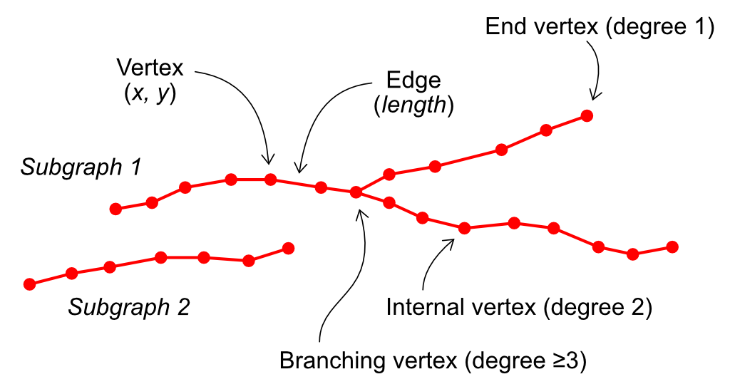
Figure 1. Euclidean graph composed by two disconnected subgraphs. Each vertex is associated with its spatial coordinates in the Euclidean plane. Each edge is associated with a weight proportional to the Euclidean distance between its vertices.

EGs accurately identify the path of curvilinear features on the original image by capturing all its salient characteristics, both topological and geometrical (e.g., branches, end points, cycles, length and form factor). Most analyses, such as the measurement of length ^[8], tortuosity ^[9], orientation ^[10] and fractal dimension ^[11][12], can therefore be performed directly on the EG itself, taking full advantage of its rich information content without resorting to the segmented image. EG representation appears also as an optimal starting point for more sophisticated analyses such as the automated pattern recognition of concrete cracks for structural assessment ^[13]. Specific analyses (such as the width measurement of a surface crack) can instead be carried out on the original grayscale image using the EG representation as a guide for precise feature localization on the image itself and for the automated selection of the parts to be measured, thus avoiding any issues related to image manipulation during the identification process. Different EGs can also be quantitatively compared according to their overlapping degree, enabling the use of well-known performance metrics, such as intersection over union and F1-scores. On top of that, the EG-based description of the curvilinear feature path provides a very convenient basis for the generation of machine-readable documentation for archiving and later analysis ^[1].

3. EG-mediated image processing

The EG-mediated automated analysis of curvilinear features in digital images can be implemented in a general approach by identifying the target features with a binary segmentation method of choice (e.g., threshold based, edge-detection based or CNNs) and then deriving a polished EG representation of the identified feature paths. The obtained EG is then available for path feature selection, direct path analysis. EG-driven analyses on the original grayscale image and for archiving or other purposes (Figure 2).

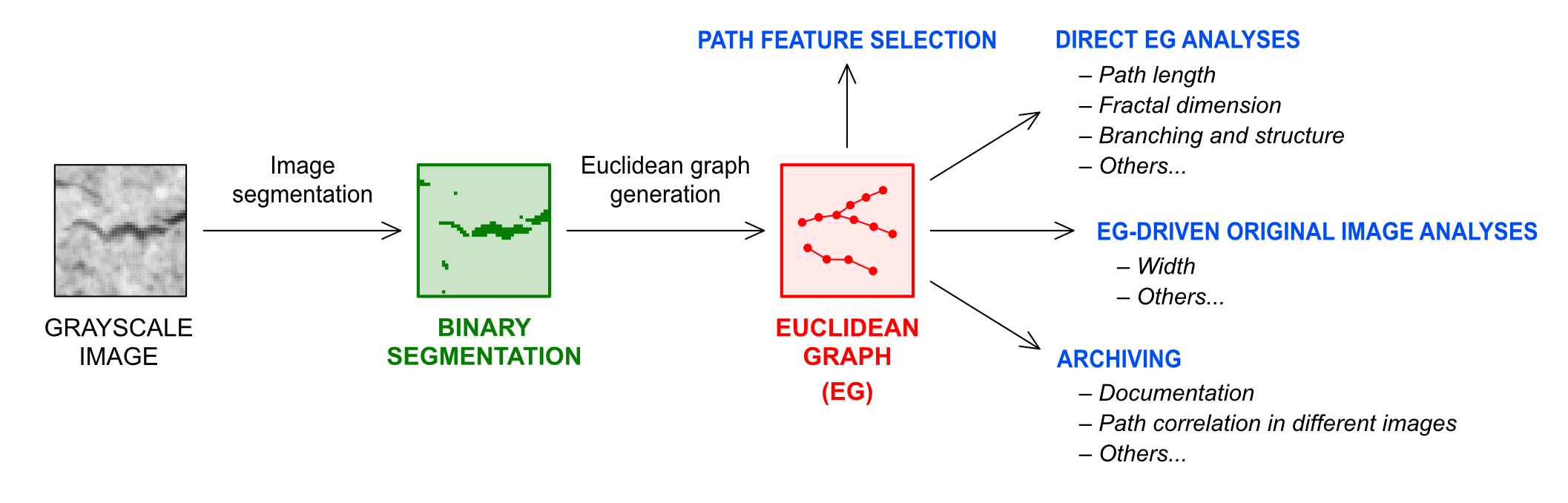
Figure 2. Fundamental steps of EG-mediated image analysis process of line-shaped features. The EG description of the feature path can be derived from any segmentation algorithm that results in a binary image, allowing the implementation of automated, highly tuned EG-based analyses to most of the existing detection methods.

The whole EG-mediated image analysis process is depicted in the flowchart of Figure 3. The image segmentation step is responsible for the primary recognition of curvilinear features, resulting in a binary image that identify the pixels putatively belonging to the target features. The binary segmented image is then skeletonized (i.e., all pixel clusters are reduced to their centerline). A raw, primal EG is directly derived from the skeletonized image with complete information retention. The primal EG is then processed in order to obtain the final EG, which is a functional description of the feature pattern captured in the original image. In a typical implementation, a strictly sequential process computes the final EG but tailored algorithms can also take advantage of direct access to the original image even in the intermediate phases, particularly in the skeletonization and EG processing steps (dashed arrows in Figure 3). Subsequent analyses can then be performed either directly on the final EG itself or on the original image using the final EG as a guide. The final EG is also functional for data archiving and comparison of curvilinear features found in different images.

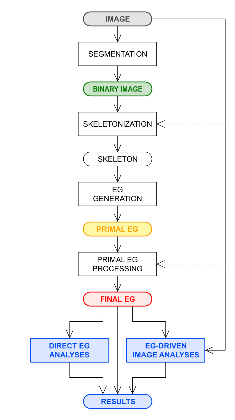
Figure 3. Complete EG-mediated image processing with primal EG generation and finishing to obtain the refined final EG suitable for downstream analyses. Advanced algorithms for skeletonization and processing of primal EG can also take advantage of the direct access to original image data.

A raw, primal EG can be derived from any binary segmented image of curvilinear objects such as cracks and other line-shaped features by skeletonization, i.e. the thinning of the feature path to a one-pixel-wide, 8-connected representation (Figure 4). The EG generation process is based on the exploration of the skeleton path with an exhaustive process analogous to the depth-first search. The complete primal EG generation algorithm is described in the supplementary information of ^[1].

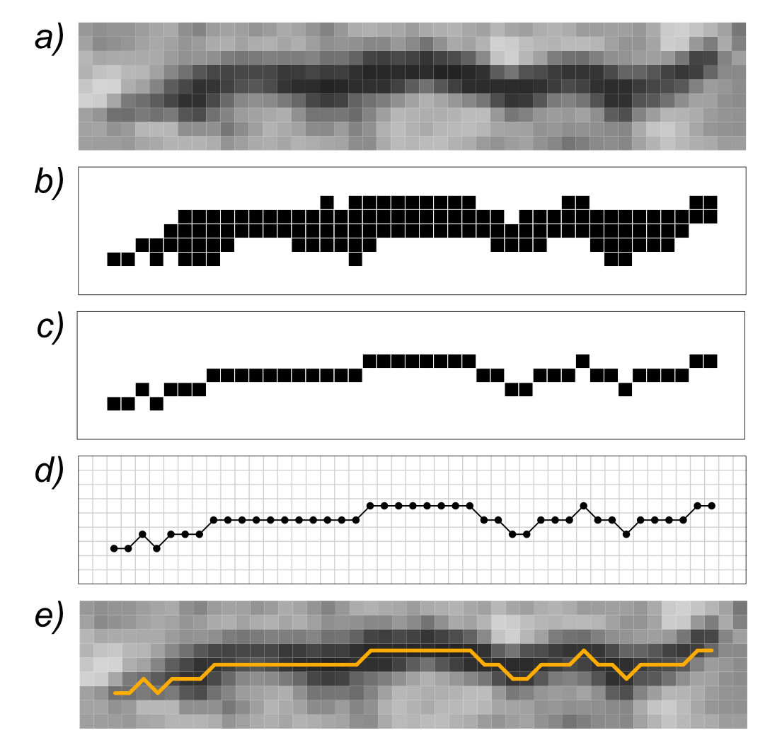
Figure 4. A grayscale image of a curvilinear feature (a) is processed with a segmentation method of choice in order to give a bitmap image (b) that is skeletonized (c). The raw EG representation (d) is directly derived from the skeletonized bitmap with full information retention. The obtained EG is shown superimposed to the original image (e).

In the primal EG, each vertex corresponds to a skeleton pixel and each edge corresponds to a neighboring pixel connection (Figure 5). The primal EG thus completely describes the skeleton path, retaining all the related information.

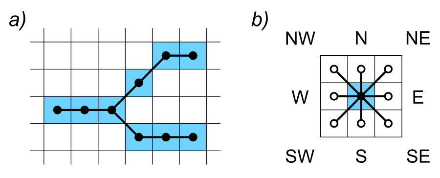
Figure 5. EG generation from skeletonized bitmap. Primal EG vertices (black dots) are uniquely correlated with skeleton pixels (depicted in blue) and are thus constrained to image pixel grids (a); edges in primal EG connect only vertices related to adjacent pixels (empty dots), here identified with compass points (b).

5. Final EG generation

In order to provide an effective functional description of the curvilinear features appearing in the image, the primal EG must be refined with a specific finishing process which can include, among the other things, noise filtering, artefacts elimination and feature merging (when there is evidence that apparently separate subgraphs are actually parts of a single, extended curvilinear object). The obtained final EG constitutes a polished representation of the curvilinear features of interest recorded in the original image.

5.1 Noise removal

The binarization of noisy images inevitably produces a considerable number of false positives (i.e., foreground pixel clusters uncorrelated to the features of interest), which can be challenging to avoid in the first place and to filter out in the post-binarization process. False positive foreground clusters subsequently translate to spurious subgraphs in the resulting EG that must be identified and removed. An example of a noisy image of a surface crack is given in Figure 6, where the primal EG shows a quite high level of noise-derived artefacts (Figure 6b). In particular, dark zones in the original image generate highly branched subgraphs that can easily include more than a hundred vertices. This rules out a simple filtration based on vertex count, requiring instead a more specific approach based on geometrical and/or topological properties. Background noise due to sample surface texture is typically characterized by small and compact pixel clusters that originate small-diameter, highly branched subgraphs. A two-step noise removal process is thus implemented in this example. The first step eliminates all subgraphs with a diameter of less than 25 px (defined as the separation of the most distant end vertices). The second step eliminates all subgraphs with a ratio between the total number of vertices and the diameter greater than 2 px⁻¹. This remarkably simple process effectively removes most part of noise artefacts (Figure 6c). A subsequent noise removal step is performed at a later stage through subgraph filtration by vertex counting which further refines the crack EG (Figure 7d).

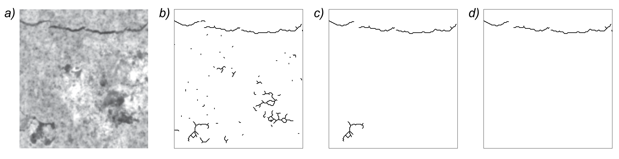
Figure 6. Noise removal with EG processing. Surface texture on a crack image (a) generates a substantial number of noise artefacts in the primal EG (b) that can be removed in later EG refining steps (c, d).

5.2 Artefact removal

The skeletonization process can generate artefacts due to local variations in the curvilinear feature thickness in the form of parasitic short branches that protrude from the skeleton path ^[14]. These translate into factitious short arms in the derived EG that must be eliminated (pruning). Additionally, spurious cycles are generated during the skeletonization when a small background pixel cluster in the segmented image (or even an isolated pixel) is completely surrounded by foreground pixels. The use of EGs allows the implementation of the morphological identification of path features based on geometrical and topological criteria that can be finely tuned according to the ongoing analysis. Specific features can then be reliably identified on the curvilinear object path for further analysis or removal. An example of EG-based artefact removal specifically tuned for crack analysis is shown in Figure 7, where a series of consecutive weighted shortest path searches based on Dijkstra’s algorithm filter out all small branches and cycle artefacts. The algorithm is fully described in the Supplementary Information of ^[1].

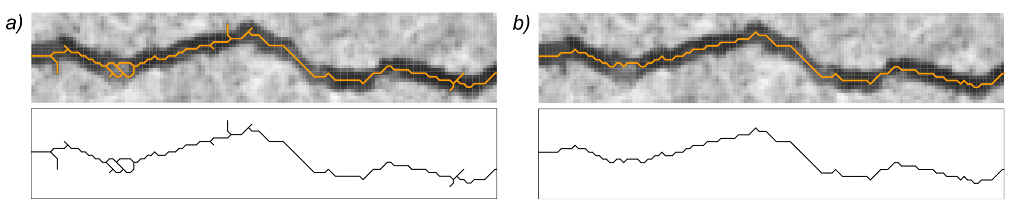
Figure 7. Artefact removal. The EG of a relatively thick crack demonstrates small branches and cycle artefacts derived from the skeletonization process (a). A removal algorithm based on shortest path search effectively removes all artefacts leaving the main crack path only (b). Top: original image with superimposed EG; bottom: EG alone.

5.3 EG Smoothing

All vertices in the primal EG are bound to specific pixels of the original digital image and are therefore localized by discrete spatial coordinates. Consequently, even if the EG path of a horizontal, vertical or 45° diagonal line is constituted by a series of aligned vertices, paths at every other inclination generate rough EGs composed of a saw-edged succession of short segments. The EG of a generic curve is thus represented by a discrete approximation made from a jagging path through the image pixel grid. This can lead to errors in some measurements carried out on pristine EG (e.g., in path length determination, where each EG deviation from the actual path causes a small positive error that accumulates in the process). However, the EG-based path representation allows to implement specific smoothing algorithms. An example based on a simple iterative algorithm ^[1] is reported in Figure 8 for a small crack image. The original EG (Figure 8b) is characterized by a strong jagging because of the direct correspondence of each vertex with a pixel in the skeletonized image. EGs derived from one, two and three smoothing cycles (Figure 8c–e, respectively) show a progressive improvement in the path evenness.

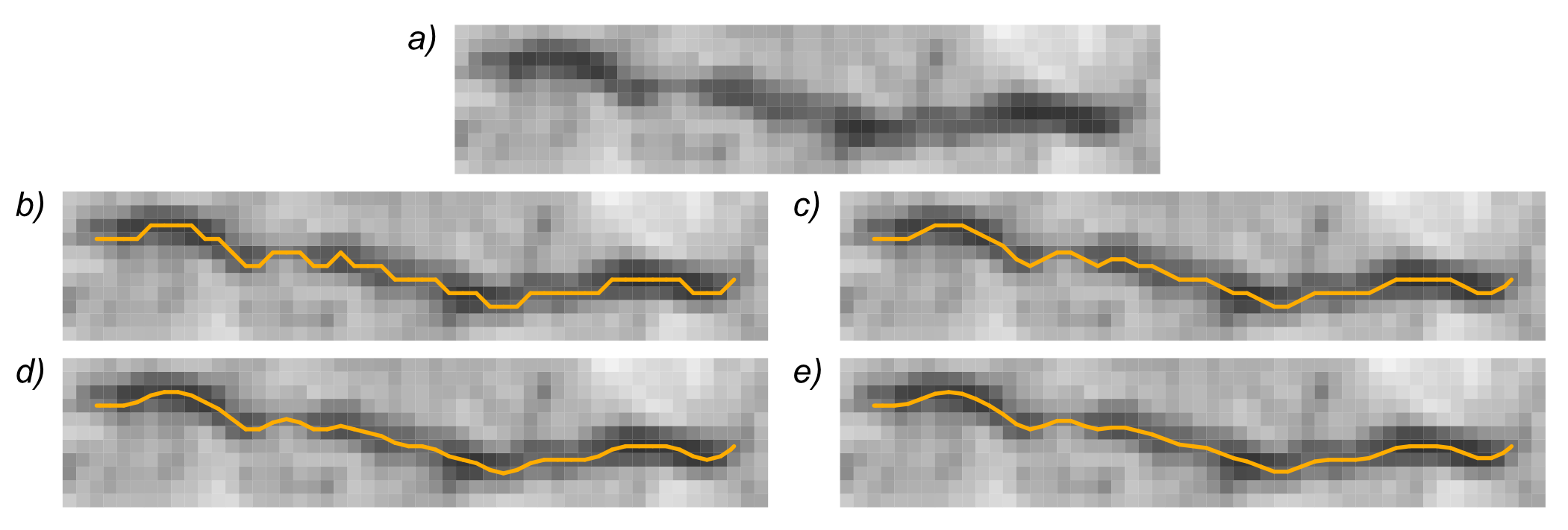
Figure 8. EG smoothing. A crack EG (b) is obtained from the original image (a) with vertices corresponding to pixel centers, resulting in a quite rough path. Paths deriving from one (c), two (d) and three (e) EG smoothing iterations, respectively, demonstrate a progressive improvement in evenness.

6. Path Selection

In the analysis of curvilinear features, it can be convenient to process selected features and even specific feature parts according to the objectives of the analysis itself. As an example, during crack width measurement, it is usually appropriate to avoid intersection and terminal zones. The availability of EG description allows an effective analysis of the curvilinear feature pattern by geometrical and topological algorithms, enabling a rational selection of the parts to be measured using objective criteria and avoiding the introduction of possible artefacts due to manipulations of the binarized image ^[1]. In the aforementioned crack width measurement, the identification of the potentially interfering zones such as crack ends or intersections can be easily accomplished on the crack EG by selecting the internal vertices that are beyond a minimum stated distance from end vertices and from branching vertices (Figure 9).

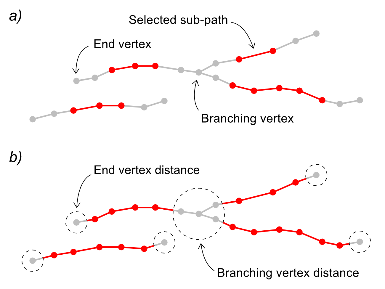
Figure 9. EG subpath selection based on distance from branching and end vertices. Selected subpaths (in red) are separated from branch and end vertices by a specified number of vertices (a) or by a predetermined geometric distance (b).

7. Quantitative Path Correlation

Two different EGs can be quantitatively compared by determining, for each of them, the part of the path that overlaps with the other. EG overlap is defined as the part of the EG path that has no distance from the path of the other EG greater than a given tolerance (Figure 10). This can be very helpful, for instance, when assessing the quality of an automated feature identification algorithms using an EG-based reference ground truth. The EG–EG comparison allows to identify the overlapping part of the EG and the ground truth EG (true positives, TP), the non-overlapping part of the final EG (false positives, FP) and the non-overlapping parts of the reference EG (false negatives, FN). The TP, FP and FN are quantified as path length on their respective EG. The values obtained can be used for the EG-based computation of performance evaluation indicators, namely precision, recall, intersection over union (IoU) and F1-score quality measures. The detailed description of EG path comparison and EG-based performance evaluation methods is reported in the Supplementary Information of ^[1].

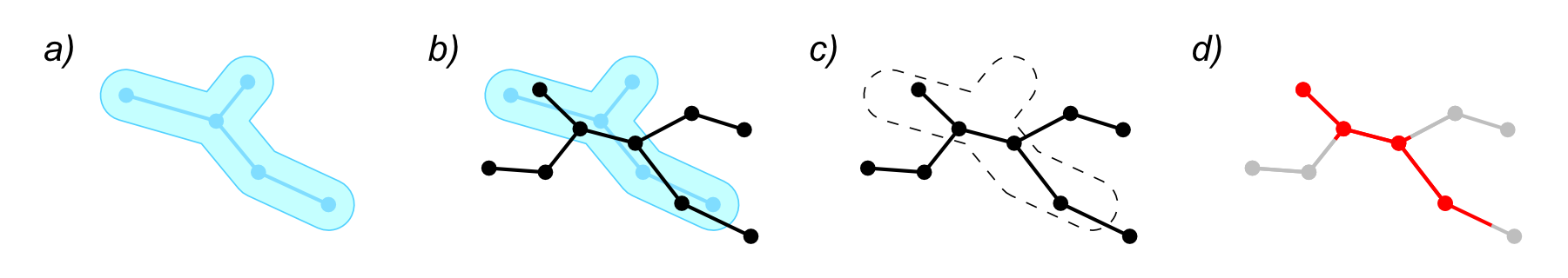
Figure 10. EG–EG path comparison. A reference EG with a defined overlap tolerance area (a). A sample EG (black) superimposed to the reference EG (b). The part of the sample EG corresponding to the reference EG falls within the overlap area while the non-matching part falls outside it (c). Sample EG with path labeled as matching (red) or non-matching (grey).

8. EG analysis

The final EG gives an effective functional description of all the curvilinear features found in the original image, each individually represented by a connected sub-EG. By describing the curvilinear features in the original image with a high resolution, the final EG allows direct EG analyses (e.g., for feature length determination) and EG-driven analyses on the original image (e.g., for feature width measurement).

8.1 Path length

The length of a curvilinear feature can be defined in several ways (e.g., as total path length or as the length of the main path). As described above, the availability of EG description allows to fine-tune the parts to be measured according to well-defined selection rules. The effective path length can then be calculated as the cumulative distance between each connected node in the EG, possibly after a smoothing process in order to reduce the errors associated with the discrete spatial nature of digital images.

8.2 Branching

Depending on the objective of the whole analysis, it can be useful to identify the main path and the secondary branches of each curvilinear feature for separate evaluation or for morphological assessment. The branch analysis can be directly derived from the final EG, for instance, by an iterative search resulting in the identification of all branches, starting from the main path and proceeding through lateral arms in decreasing length order ^[1]. Furthermore, the same algorithm allows to classify the lateral branches observed during the analysis as primary (if directly connected to the main path), secondary (if connected to a primary branch) and so on (Figure 11).

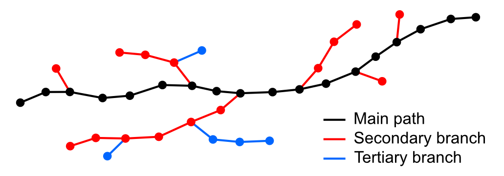
Figure 11. EG with identified main path (black) and lateral branches (red and blue). The latter can also be classified by length or by the connection hierarchy as depicted in the figure.

8.3 Crack width

A very common requirement in crack analysis is the determination of the crack width. There are several definitions of crack width in the literature, either global or local ^[1]. The definition of a local crack width, giving the best results in most contexts ^[9], is the distance of the intersection points of the crack boundaries from a line perpendicular to the tangent of a given point of the central line ^[15]. With the availability of the EG description of the crack path, this method can be implemented very conveniently by computing the tangent line of a given EG vertex by linear fitting of neighboring vertex positions. The crack width is then evaluated on the original image along a measurement line perpendicular to the tangent line and passing through the involved vertex. A slightly different approach that is appropriate, for example in the case of constant strain direction ^[1], entails the use of parallel measurement lines at a fixed orientation (typically given by the strain vector). Crack EGs also make this approach very practical, as it may be implemented by defining a series of parallel equidistant lines and then finding the intersection point between these latter lines and the EG itself (Figure 12).

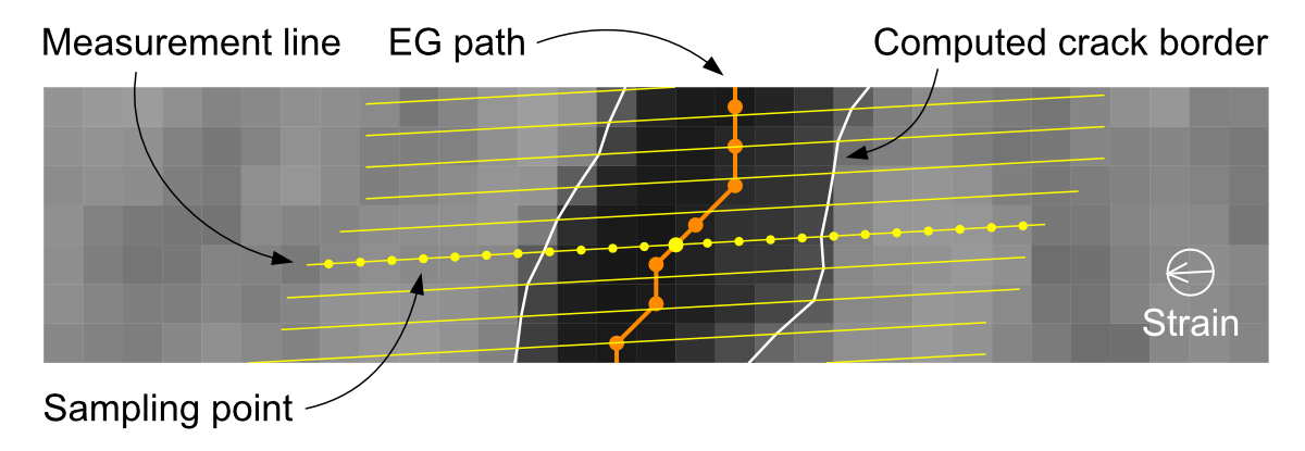
Figure 12. EG-driven crack width determination on the original grayscale image with parallel measurement lines along the strain direction (yellow). The center of each measurement line (thicker yellow dot) is located at the intersection with the crack EG path (orange).

9. Advantages

EG-mediated curvilinear feature analysis has several advantages over traditional analysis methods based on binary segmentation due to its information richness, computational efficiency and wide implementation possibilities, as detailed below.

Information richness. The topological and geometrical information conveyed by EGs allows the implementation of tailored algorithms for the refinement of the detected curvilinear features and for their selection, classification, processing and analysis. These algorithms are usually more efficient than their counterpart based on segmented binary images and, in many cases, they can be implemented only with an EG-based object path description.

Feature selection. Particular features and feature parts can be algorithmically identified and classified on the EG itself according to specific requirements. Feature selection procedures can thus be implemented with well defined and objective criteria.

Feature localization on the original image. The positional information associated with each EG vertex allows a precise localization on the original image for specific measurement tasks. Special analyses (e.g., accurate width determination in surface crack detection) can therefore be implemented directly on the original image avoiding potential pitfalls due to previous image binarization and manipulation processes.

Feature comparison. The EG description of the curvilinear features identified in different images can be used as a basis for quantitative comparison analysis (e.g., in time evolution studies). Moreover, quantitative path correlation between EGs can be performed using well-known performance evaluation methods (e.g., intersection over union and F1-score).

Archiving. EGs can be the foundation for a machine-readable, high-resolution documentation for archiving and later analysis. Moreover, the high information richness of EGs offers great opportunities for data compression maintaining the essential features of the described path (e.g., by removing selected, uninformative internal nodes while keeping all branching and end nodes).

Computational efficiency. The skeletonized image is explored only once during the EG generation, then all of the related information is recorded in the EG and made widely available for computational purposes in later processes. This ensures, for example, a very efficient retrieval of special features (e.g., branching points) that would otherwise have to be searched every time on the segmented image (a computationally expensive process).

Implementation potential. EGs can be easily derived from any binary-segmented image, ensuring a wide implementation potential. The EG representation of curvilinear features therefore constitutes an ideal interface between any detection algorithm resulting in a binary segmentation (e.g., threshold binarization and CNNs) and the following post-detection analysis processes.

This entry is adapted from the peer-reviewed paper 10.3390/s22165942

References

- Strini A.; Schiavi L.; Euclidean Graphs as Crack Pattern Descriptors for Automated Crack Analysis in Digital Images. Sensors 2022, 22, 5942, 10.3390/s22165942.
- Koch, C.; Georgieva, K.; Kasireddy, V.; Akinci, B.; Fieguth, P.; A review on computer vision based defect detection and condition assessment of concrete and asphalt civil infrastructure. Adv. Eng. Inform. 2015, 29, 196-201, 10.1016/j.aei.2015.01.008.
- Jahanshahi, M.R.; Chen, F.C.; Joffe, C.; Masri, S.F.; Vision-based quantitative assessment of microcracks on reactor internal components of nuclear power plants. Struct. Infrastruct. Eng. 2017, 13, 1013–1026, 10.1080/15732479.2016.1231207.
- Jan, J., Odstrcilik, J., Gazarek, J., Kolar, R.; Retinal image analysis aimed at blood vessel tree segmentation and early detection of neural-layer deterioration. Comput. Med. Imaging Graph. 2012, 36, 431–441, 10.1016/j.compmedimag.2012.04.006.
- Acciai, L.; Costantini, I.; Pavone, F.S.; Conti, V.; Guerrini, R.; Soda, P.; Iannello, G.; Towards automated neuron tracing via global and local 3D image analysis. IEEE 13th International Symposium on Biomedical Imaging (ISBI) 2016,
, 322–325, 10.1109/isbi.2016.7493274. - Carlotto, M.J.; Enhancement of Low-Contrast Curvilinear Features in Imagery. IEEE Trans. Image Process. 2007, 16, 221-228, 10.1109/tip.2006.884949.
- Vicas, C.; Nedevschi, S.; Detecting Curvilinear Features Using Structure Tensors. IEEE Trans. Image Process. 2015, 24, 3874–3887, 10.1109/tip.2015.2447451.
- Yu, S.N.; Jang, J.H.; Han, C.S.; Auto inspection system using a mobile robot for detecting concrete cracks in a tunnel. Autom. Constr. 2007, 16, 255–261, 10.1016/j.autcon.2006.05.003.
- Berrocal, C.G.; Lofgren, I.; Lundgren, K.; Gorander, N.; Hallden, C.; Characterisation of bending cracks in R/FRC using image analysis. Cem. Concr. Res. 2016, 90, 104–116, 10.1016/j.cemconres.2016.09.016.
- Arena, A.; Delle Piane, C.; Sarout, J.; A new computational approach to cracks quantification from 2D image analysis: Application to micro-cracks description in rocks. Comput. Geosci. 2014, 66, 106–120, 10.1016/j.cageo.2014.01.007.
- Yao, J.W.; Chen, J.K.; Lu, C.S.; Fractal cracking patterns in concretes exposed to sulfate attack. Materials 2019, 12, 2338, 10.3390/ma12142338.
- Rezaie, A.; Mauron, A.J.P.; Beyer, K.; Sensitivity analysis of fractal dimensions of crack maps on concrete and masonry walls. Autom. Constr. 2020, 117, 103258, 10.1016/j.autcon.2020.103258.
- Liu, Y.; Yeoh, J.K.W.; Automated crack pattern recognition from images for condition assessment of concrete structures. Autom. Constr. 2021, 128, 103765, 10.1016/j.autcon.2021.103765.
- Saha, P.K.; Borgefors, G.; de Baja, G.S.. Skeletonization - Theory, Methods, and Applications; Academic Press: London, 2017; pp. 22–23, 131–135.
- Carrasco, M.; Araya-Letelier, G.; Velazquez, R.; Visconti, P.; Image-based automated width measurement of surface cracking. Sensors 2021, 21, 7534, 10.3390/s21227534.