Your browser does not fully support modern features. Please upgrade for a smoother experience.
Please note this is an old version of this entry, which may differ significantly from the current revision.
Subjects:
Water Resources
Groundwater level (GWL) refers to the depth of the water table or the level of water below the Earth’s surface in underground formations. It is an important factor in managing and sustaining the groundwater resources that are used for drinking water, irrigation, and other purposes. Groundwater level prediction is a critical aspect of water resource management and requires accurate and efficient modelling techniques.
- groundwater levels (GWL)
- machine learning
- deep learning
1. Physically Based Numerical Method—MODFLOW
Physically based numerical models remain the best methods to study the characteristics of groundwater. This is because they require comprehensive details of the physical properties of aquifer. Among the different physically based numerical models, MODFLOW is the most used model in the literature; it models groundwater movement in three dimensions using finite differences. Until the last decade, MODFLOW was used extensively, especially when sufficient data are not available. Depending upon the problem, several approaches are designed for MODFLOW, i.e., the head-oriented approach (HOA) is used to determine the three-dimensional flow of groundwater, the velocity-oriented approach (VOA) comes in handy when computing the velocity of flowing groundwater [48]. However, certain steps are needed to formulate such a model, i.e., grid design, boundary setting, time steps, and hydrologic and aquifer characteristic variables selection. Shukla and Singh [49] calibrated MODFLOW in Uttar Pradesh, India to simulate groundwater levels. Data mostly comprising of water levels collected between 2005 and 2013 were used in the study. In addition, the impact of pumping and recharge rate on the groundwater levels was also studied, and it aimed to predict the groundwater levels for five years ahead. The results showed a declining trend in groundwater levels in the region.
2. Machine Learning—Artificial Neural Networks (ANN)
ANN is computational representation of a mathematical model inspired by the human brain’s biological network. Simple elements called neurons, operating in parallel, constitute ANN [50]. ANNs are used to calculate unknown functions or to make future predictions of the given time series based on historical data. The most basic ANN is a three-layer structure, with input, hidden, and output layers [51]. The structural representation of classical FFNN into the network and the desired outcome is computed by the output layer. The hidden layer nodes which are situated between the input and output layers receive a set of scaled inputs and calculate an output after applying a certain learning (activation) function [52].
A sample dataset Is used to train the ANN model. Training is a process of fine-tuning the network’s adjustable parameters (known as weights and biases) to optimize the output of the algorithm. “The Levenberg-Marquardt (LM) algorithm, the backpropagation (BP) algorithm, the Bayesian regularization (BR) algorithm, and the gradient descent with momentum and adaptive learning rate back-propagation (GDX) algorithm” are some learning algorithms that have been employed to train models in the literature. Feed-forward neural networks (FFNNs), usually known as multilayer perceptrons (MLPs), are a popular and robust type of ANN that has been widely studied in hydrological studies [53]. Figure 4 shows the different kinds of data used for prediction the GWL.
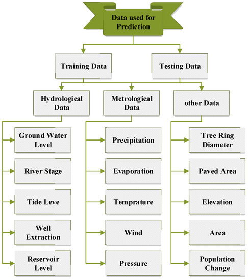
Figure 4. Different kinds of data used for prediction of GWL.
ANNs have been widely used in hydrology, hydraulics, rainfall-runoff estimation, groundwater level, and quality forecasting [54,55,56]. According to recent GWL modeling studies, it has been reported that ANN simulations have shown promising results compared to conceptual techniques. In one of the first studies, Lallahem et al. [4] used ANNs to simulate monthly groundwater (GWL) for an aquifer. Inputs included evapotranspiration, averaged temperature, precipitation, rainfall, and GWL at the previous lag of 13 piezometers and the primary objective was to anticipate GWL for a specific piezometer in northern France. The advantage of the multi-layer perceptron MLP was proven by simulation results. Krishna et al. [57] compared several types of FFNNs to simulate the monthly GWL in Andhra Pradesh urban aquifer, India. Results revealed the merit of an ANN trained with the LM algorithm as compared to BP and BR algorithms. Moreover, in the experiment, the best-performing network model parameters were used to predict the GWL in nearby wells.
Sreekanth et al. [5] developed ANFIS and FFNN with an LM algorithm to estimate GWL for India’s Maheshwaram watershed. Monthly groundwater (GWL) of 22 wells, rainfall, temperature, evaporation, and relative humidity are among the input variables. FNN outperformed ANFIS in terms of accuracy when results were compared. Kouziokas et al. [58] compared multiple FFNN networks and learning methods to simulate the daily groundwater (GWL) in a well. The study area is located in Montgomery County, Pennsylvania, USA. The best model was found to be FFNN trained using the LM learning algorithm with the humidity, precipitation, and temperature as inputs.
3. Adaptive Neuro-Fuzzy Inference System (ANFIS)
This is a hybrid technique that aims to utilize the advantage of a fuzzy inference system (FIS) with an adaptable neural network (AN). FIS is based on fuzzy logic and is good at capturing uncertainties and noise in data. Jang [59] pioneered the use of fuzzy if–then rules with right membership functions (MPs) to construct input–output pairs and a neural network learning algorithm. The fuzzy inference aystem is further classified into two approaches, namely Mamdani and Sugeno. Linear MFs are used by the Sugeno approach while Mamdani uses fuzzy MFs. ANFIS consists of five layers. The structural representation of ANFIS is similar to the ANN model, except it has two input parameters, linear and non-linear, which makes it difficult to train. Input parameters are optimized simultaneously in the training process.
Zhang et al. [60] applied three different algorithms for GWL prediction, namely, radial basis function neural network (RBFNN), ANFIS, and the grey self-memory (GSM) method. Evaluation reveals the superiority of ANFIS over the other applied algorithms based on the performance metrics result (i.e., NSE, RMSE, R2, and MARE). Bak and Bae [61] trained the ANFIS algorithm with precipitation (P) and mean temperature (Tmean) to predict GWL and reported the performance metrics RMSE as 0.1381 and MAPE as 37.869%.
Gong et al. [62] investigated the prediction accuracy of ANFIS, FNN, and SVM for monthly GWL simulation and concludes the superiority of ANFIS over other algorithms. Previous GWL, lake level, precipitation (P), and Tmean were used as input variables. Khaki et al. [63] investigated the performance of ANFIS, FFNN, and the cascade forward network (CFN) model to simulate monthly GWL at Langat Basin in Selangor state’s southeastern part. R and MSE were used as performance metrics. The ANFIS model outperformed FFNN and CFN with R = 0.94 and MSE = 0.005. Emamgholizadeh et al. [64] analyzed the differences in the monthly GWL prediction of ANN and ANFIS in Bastam plain, Iran. The following input variables were used in the study: pumping rate, rainfall recharge, and irrigation returned flow. ANFIS performed significantly better than ANN and it was also found that high accuracy can be achieved by applying different structures. Sometimes, hydrological time series data can be highly non-stationary which makes it hard for models, such as ANN and ANFIS, to better understand the underlying seasonality and thus leads to inaccurate predictions. In this situation, some researchers, such as Hsu and Li [65] and Loboda et al. [66], applied the wavelet data decomposition technique to first pre-process the input data. Wavelet transform can decompose data at various resolution levels to obtain useful information and give insights about trends and irregularities in the data. Therefore, it has several applications in hydrological studies because of the non-stationary nature of the data.
The performance of regular ANNs, ANFISs, and both coupled with the wavelet technique, i.e., WANN and WANFIS, was examined by Moosavi et al. [67]. They conducted a study to simulate monthly GWL for two subbasins in Mashad, Iran. Precipitation (P), evaporation (E), temperature (T), and previous GWL were the input variables. ANN and ANFIS failed to cope with the noise in the data while the ones coupled with wavelet performed considerably better. However, the authors reported that wavelet transform does contribute more to the efficiency of ANFIS than ANN. Another study was performed by Ebrahimi and Rajaee [68] to analyze the impact of the wavelet pre-processing technique. They developed wavelet-ANN, multi-linear regression (wavelet-MLR), and support vector machine (wavelet-SVM) up to two decomposition levels, and their regular counterparts. GWL at previous lag was used as the only input variable to simulate GWL with a one-month lead. The results showed that data decomposition translates into the high prediction accuracy of the models. Nevertheless, wavelet-ANN is reported as the best model. Machine learning models using prior wavelet data decomposition are good at yielding underlying trends and patterns at various levels in non-linear and non-stationary input data. Figure 5 shows the basic architecture of ANFIS model.
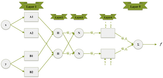
Figure 5. A basic architecture of ANFIS model.
4. Genetic Programming (GP)
A general genetic algorithm (GA) was developed called genetic programming (GP) [69]. Darwinian theories of evolution are used for genetic programming and ecological choice as the GA. The author in [70] developed a GP-based model to predict the GWL changes and calculate the vagueness in the forecasting. The paper used Indian monthly rainfall data to predict the GWL. The GP model proposed by the author could successfully predict variations by using only hydrometeorological parameters for GWL, i.e., the model predicts without knowing the physical characteristics of the wells. GP has been mostly affected for feature selection work and optimization. Furthermore, because of its flexibility and intelligible tree structure it is more used in GW modeling. The author in [71] proposed GWL for the next day and prediction intervals of up to 7 days and applied SVM, GP, ANN, and ANFIS. All of these algorithms have prediction capabilities to predict GWL. There are several GWL combinations, including evapotranspiration and rainfall data, which are used as input to the prediction model, using data gathered from Republic of Korean, Hongcheon well station. After making a model, the autoregressive moving average (ARMA) model is used for comparison to validate the accuracy. The final conclusions proved that the ARMA methodology performed well compared to other ML methods, which is therefore the most effective with the GP model.
5. Deep Learning
Despite the significant performances of ANN and ANFIS in accurately predicting the GWL, these methods were confined by the vanishing and exploding gradient problem, thus hindering the capability of the machine learning models to make predictions for long-time series. A recurrent neural network (RNN) is a type of neural network that was introduced to solve the long-term dependency problem when dealing with large-scale data in the temporal domain. However, regular RNN cannot remember temporal information for long sequences, i.e., in the machine translation tasks, etc., and require large computational resources. To overcome the limitations of regular RNN, the long short-term memory (LSTM) model was proposed to keep the information for an arbitrary length. LSTM is mainly developed for continuous data—time-series data. Recently, it has been employed in various water level assessment studies.
Zhang et al. [6] proposed the LSTM model to simulate the fluctuations in water table levels using monthly water diversion, precipitation, evaporation, temperature, and previous water table level data spanning 14 years (2000–2013). The results achieved were dramatically high (R2 score, 0.789) when compared with the R2 scores (0.004–0.495) of the traditional feed-forward neural network (FFNN or regular ANN). To select relevant predictors, the authors used a statistical technique that contributed to the model’s ability to generalize from the unseen data. The study was performed in five sub-areas of Hetao, China. GWL fluctuations data are prone to the existence of missing values because of several factors, i.e., human negligence, failure of recording equipment, etc. Gaps in data can make it difficult to grasp the hidden trends and seasonality. Therefore, this has led the missing values being reconstructed to fully interpret the data and make accurate predictions so that strategists can make plans for water resource management in the long run. Ren et al. [72] evaluated the ability of an LSTM model against a traditional gap-filling algorithm, ARIMA, to fill missing temporal observations for a 10-year-long dataset with dynamic gaps. The model was designed to reconstruct specification measurements (groundwater and river water interactions). The results revealed that LSTM is better at filling high dynamic gaps (daily, weekly, and sub-daily), while ARIMA excelled in reconstructing trends and seasonality-based gaps. In addition, the authors reported that LSTM can fill gaps for up to 2 days when spatial data from neighboring stations are used to make predictions. Table 1 presents detail research categorized by different algorithms: deep learning, GP, MODFLOW, ANFIS, and ANN.
Table 1. Research categorized by different algorithms: deep learning, GP, MODFLOW, ANFIS, ANN.
| References | Deep Learning | GP | MODFLOW | ANFIS | ANN |
|---|---|---|---|---|---|
| P. Shukla and R. M. Singh [49] | ✓ | ||||
| Lallahem et al. [4] | ✓ | ||||
| Krishna et al. [56] | ✓ | ||||
| Sreekanth et al. [5] | ✓ | ✓ | |||
| Kouziokas et al. [57] | ✓ | ||||
| Zhang et al. [62] | ✓ | ||||
| Gong et al. [55] | ✓ | ✓ | |||
| Khaki et al. [64] | ✓ | ✓ | |||
| Emamgholizadeh et al. [65] | ✓ | ✓ | |||
| Kasiviswanathan et al. [69] | ✓ | ||||
| Shiri et al. [71] | ✓ | ||||
| Zhang et al. [6] | ✓ | ✓ | |||
| Ren et al. [72] | ✓ | ||||
| bowes et al. [73] | ✓ | ||||
| Shin et al. [74] | ✓ | ||||
| Javadinejad et al. [75] | ✓ | ||||
| Moravej et al. [76] | ✓ | ||||
| Khedri et al. [77] | ✓ | ||||
| Seifi et al. [78] | ✓ | ||||
| Demirci et al. [79] | ✓ | ✓ | |||
| Djurovic et al. [80] | ✓ | ||||
| Jalalkamali et al. [81] | ✓ | ||||
| Zeydalinejad et al. [2] | ✓ | ||||
| Mukherjee et al. [32] | ✓ | ||||
| Moosavi et al. [68] | ✓ | ||||
| Sun et al. [82] | ✓ | ||||
| Ghose et al. [83] | ✓ | ||||
| Shan et al. [84] | ✓ | ✓ | |||
| Ghasemlounia et al. [85] | ✓ | ||||
| Yin et al. [86] | ✓ |
This entry is adapted from the peer-reviewed paper 10.3390/app13042743
This entry is offline, you can click here to edit this entry!