Your browser does not fully support modern features. Please upgrade for a smoother experience.
Please note this is an old version of this entry, which may differ significantly from the current revision.
Subjects:
Others
The functionality of a protein is dependent upon its structure, and structure-based drug design (SBDD) relies on the 3D structural information of the target protein, which can be acquired from experimental methods, such as X-ray crystallography, NMR spectroscopy and cryo-electron microscopy (cryo-EM). The aim of SBDD is to predict the Gibbs free energy of binding (ΔGbind), the binding affinity of ligands to the binding site, by simulating the interactions between them.
- drug discovery
- computer-aided drug design
- in silico drug design
1. Introduction
New drugs with better efficacy and reduced toxicity are always in high demand, however the process of drug discovery and development is costly and time consuming and presents a number of challenges. The pitfalls of target validation and hit identification aside, a high failure rate is often observed in clinical trials due to poor pharmacokinetics, poor efficacy, and high toxicity [1,2]. A study conducted by Wong et al. that analysed 406,038 trials from January 2000 to October 2015 showed that the probability of success for all drugs (marketed and in development) was only 13.8% [3]. In 2016, DiMasi and colleagues [4] estimated a research and development (R&D) cost for a new drug of USD $2.8 billion based upon data for 106 randomly selected new drugs developed by 10 pharmaceutical companies. The average time taken from synthesis to first human testing was estimated to be approximately 2.6 years (31.2 months) and cost approximately USD $430 million, and from the start of a clinical testing to submission with the FDA was 6 to 7 years (80.8 months). In comparison to a study conducted by the same author in 2003, the R&D cost for a new drug had increased drastically by more than two-fold (from USD $1.2 billion) [5]. A possible reason for the increase in R&D cost is that regulators, such as the FDA have become more risk averse, tightening safety requirements, leading to higher failure rates in trials and increased costs for drug development. It is therefore important to optimise every aspect of the R&D process in order to maximise the chances of success.
The process of drug discovery starts with target identification, followed by target validation, hit discovery, lead optimisation, and preclinical/clinical development. If successful, a drug candidate progresses to the development stage, where it passes through different phases of clinical trials and eventually submission for approval to launch on the market (Figure 1) [6].
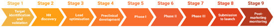
Figure 1. Stages of drug discovery and development.
Briefly, drug targets can be identified using methods, such as data-mining [7], phenotype screening [8,9], and bioinformatics (e.g., epigenetic, genomic, transcriptomic, and proteomic methods) [10]. Potential targets must then be validated to determine whether they are rate limiting for the disease’s progression or induction. Establishing a strong link between the target and disease builds up confidence in the scientific hypothesis and thus greater success and efficiency in later stages of the drug discovery process [11,12].
Once the targets are identified and validated, compound screening assays are carried out to discover novel hit compounds (hit-to-lead). There are various strategies that can be used in this screening, involving physical methods, such as mass spectrometry [13], fragment screening [14,15], nuclear magnetic resonance (NMR) screening [16], DNA encoded chemical libraries [17], high throughput screening (HTS) (such as protein or cells) [18] or in silico methods, such as virtual screening (VS) [19].
After hit compounds are identified, properties, such as absorption, distribution, metabolism, excretion (ADME), and toxicity should be considered and optimised early in the drug discovery process. Unfavourable pharmacokinetic and toxicity profile of a drug candidate is one of the hurdles that often leads to failure in the clinical trials [20].
Although physical and computational screening techniques are distinct in nature, they are often integrated in the drug discovery process to complement each other and maximise the potential of the screening results [21].
Computer-aided drug design (CADD) utilises this information and knowledge to screen for novel drug candidates. With the advancement in technology and computer power in recent years, CADD has proven to be a tool that reduces the time and resources required in the drug discovery pipeline.
2. Structure-Based Drug Design
The functionality of a protein is dependent upon its structure, and structure-based drug design (SBDD) relies on the 3D structural information of the target protein, which can be acquired from experimental methods, such as X-ray crystallography, NMR spectroscopy and cryo-electron microscopy (cryo-EM). The aim of SBDD is to predict the Gibbs free energy of binding (ΔGbind), the binding affinity of ligands to the binding site, by simulating the interactions between them. Some examples of SBDD include molecular dynamics (MD) simulations [22], molecular docking [23], fragment-based docking [24], and de novo drug design [25]. Figure 3 describes a general workflow of molecular docking that will be discussed in greater detail.
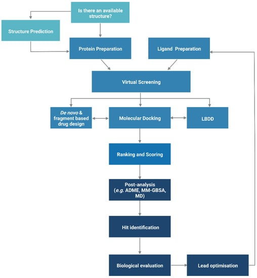
Figure 3. General workflow of molecular docking. The process begins with the preparation of the protein structure and ligand database separately, followed by molecular docking in which the ligands were ranked based on their binding pose and predicted binding affinity. (Abbreviations: LBDD: Ligand-based drug design; ADME: absorption, distribution, metabolism and excretion; MD: molecular dynamics; MM-GBSA: molecular mechanics with generalised Born and surface area).
2.1. Protein Structure Prediction
The advancements in sequencing technology led to a steep increase in recorded genetic information thus rapidly widening the gap between the amounts of sequence and structural data available. As of May 2022, the UniprotKB/TrEMBL database contained over 231 million sequence entries, yet there are only approximate 193,000 structures recorded in the Protein Data Bank (PDB) [26,27]. To model the structures of those proteins where structural data is not available, homology (comparative) modelling or ab initio methods can be used.
2.1.1. Homology Modelling
Homology modelling involves predicting the structure of a protein by aligning its sequence to a homologous protein that serves as a template for the construction of the model. The process can be broken down into three steps: (1) template identification, (2) sequence-template alignment, and (3) model construction.
Firstly, the protein sequence is obtained, either experimentally or from databases, such as the Universal Protein Resource (UniProt) [28], and this is followed by identifying modelling templates that have high sequence similarity and resolution by performing a BLAST [29] search against the Protein Data Bank [30]. PSI-BLAST [29] uses profile-based methods to identify patterns of residue conservation, which can be more useful and accurate than simply comparing raw sequences, as protein functions are predominately determined by the structural arrangement rather than the amino acid sequence. One of the biggest limitations of homology modelling is that it relies heavily upon the availabilities of suitable templates and accurate sequence alignment. A high sequence identity between the query protein and the template normally gives greater confidence in the homology model. Generally, a minimum of 30% sequence identity is considered to be a threshold for successful homology modelling, as approximately 20% of the residues are expected to be misaligned for sequence identities below 30%, leading to poor homology models. Alignment errors are less frequent when the sequence identity is above 40%, where approximately 90% of the main-chain atoms are likely to be modelled with a root-mean-square deviation (RMSD) of ~1 Å, and the majority of the structural differences occur at loops and in side-chain orientations [31].
Pairwise alignment methods are used when comparing two sequences and they are generally divided into two categories—global and local alignment (Figure 4). Global alignment aims to align the entire sequences and are most useful when sequences are closely related or of similar lengths. Tools such as EMBOSS Needle [32] and EMBOSS Stretcher [32] use the Needleman–Wunsch algorithm [33] to perform global alignment. In comparison to using a somewhat brute-force approach, the Needleman–Wunsch algorithm uses dynamic programming to find the best alignment by reducing the number of possible alignments that need to be considered and guarantees to find the best alignment. Dynamic programming aims to break a larger problem (the entire sequence) into smaller problems which are then solved optimally. The solutions to these smaller problems are then used to construct an optimal solution to the original problem [34]. The Needleman–Wunsch algorithm first builds a matrix that is subjected to a gap penalty (negative scores in first row and column), and the matrix is used to assign a score to every possible alignment (usually positive score for match, no score or penalty for mismatch and gaps). Once the cells in the matrix are filled in, traceback starts from the lower right towards the top left of the matrix to find the best alignment with the highest score.
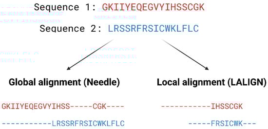
Local alignment, on the other hand, aims to identify regions that share high sequence similarity, which is more useful when aligning sequences that are dissimilar or distantly related. EMBOSS water [32] and LALIGN [32] are tools that use the Smith–Waterman algorithm [35] for local alignment. The Smith–Waterman algorithm, such as the Needleman-Wunsch algorithm, uses dynamic programming to perform sequence alignment. However, there is no negative score assigned in this algorithm, and the first row and column are set to 0. Traceback begins with the matrix cell from the highest score and travels up/left until it reaches 0 to produce the highest scoring local alignment.
When searching for templates used for homology modelling, including multiple sequences will improve accuracy of the alignment in regions where there is a low sequence homology, hence multiple sequence alignment (MSA) is essential. The global alignment method for multiple sequences is generally too computationally expensive; modern MSA tools (e.g., ClustalW [36], T-Coffee [37] and MUSCLE [38]) commonly use a progressive alignment approach that combines global and/or local alignment methods, followed by the branching order of a guide tree. This technique aims to achieve a succession of pairwise alignments, first aligning the most similar sequences and then progressing to the next most similar sequence until the entire query set has been incorporated.
For example, MSA was used during the construction of the homology models for Alanine-Serine-Cysteine transporter (SLC1A5) by Garibsingh et al. At the time, there was limited structural information on SLC1A5 due to the lack of an experimentally determined structure of human SCL1 family proteins. Most of the knowledge on the human SLC1 family protein therefore came from the study of prokaryotic homologs, which share low sequence identity. Using the structural information of the recently solved human SLC1A3, Garibsingh et al. carried out a phylogenetic analysis by generating MSA of the human SCL1 family and its prokaryotic homologs using MUSCLE and Promals3D [39], and built two different conformations of SLC1A5 homology models for the design of SLC1A5 inhibitors [40].
Once the alignment is complete, the model can be constructed starting with the backbone, then loops and lastly side-chains. The polypeptide backbone of the protein is first created by copying the coordinates of the residues from the template to create the model backbone. Gaps between the alignment of the sequence and the template are then taken care of through insertions and deletions in the alignment. It is important to remodel gaps accurately, as any error introduced here, will be amplified in later stages, thus leading to structural changes that can be critical for protein functionality and protein–protein interactions. Loop modelling, via knowledge-based methods or energy-based methods, can be used to generate predictions of the conformations of the loop. Knowledge-based methods look for experimental data on loops with high sequence similarity to the target from databases, such as PDB, and then insert them into the model. Yang et al. used FREAD [41] to predict the structure of a missing loop and construct a model of a monoclonal antibody, Se155-4, to study its antibody–antigen interactions with Salmonella Typhimurium O polysaccharide [42]. On the other hand, energy-based methods predict protein folding using ab initio methods with scoring function optimisation. For example, the Rosetta Next-Generation Kinematic Closure protocol [43], which employs the ab initio method, was used in loop prediction calculations to construct parts of the leucine-rich repeat kinase 2 (LRRK2) model, as the homology model template had missing loop sections. Mutations in the catalytic domains of LRRK2 are associated with familial and sporadic Parkinson’s disease, yet little is known about its overall structure and the mutations, which alter LRRK2 function and enzymatic activities. Combining homology models with experimental constraints, Guaitoli and co-workers constructed the first structural model of the full length LRRK2 that includes domain engagement and contacts. The model provided insight into the roles that the different domains play in the pathogenesis of Parkinson’s disease and will serve as a basis for future drug design on LRRK2 [44].
Lastly, side-chains are built onto the backbone model according to the target sequence. Most side-chain types in proteins have a limited number of conformations (rotamers) and programs such as SCWRL [45] predict these in order to minimise the total potential energy. Upon completion, the model is optimised using molecular mechanics force fields to improve its quality.
A ligand-based approach can be utilised to further optimise homology models with low sequence identity between query sequence and structural template. Moro et al. first presented ligand-based homology modelling, also known as ligand-guided or ligand-supported homology modelling, as a tool to inspect G protein-coupled receptors (GPCRs) structural plasticity [46]. GPCRs comprise a superfamily of membrane proteins with over 800 members; they play a significant role in cellular signalling in the human body. As such, GPCRs are associated with numerous biological processes, making them important therapeutic targets [47]. Unfortunately, crystallisation of membrane proteins is known to be challenging, especially in the case of GCPRs, and there were few structural data of GPCRs available until the last decade.
Given that the GPCRs are a diverse family, additional optimisation is required to refine homology models built for those with low sequence identity to the structural template to increase the level of accuracy. In this approach, an initial homology model is first developed using the conventional method. Active ligands are then docked into the binding site for optimisation. The receptor is reorganised and refined based upon the ligand binding in order to better accommodate ligands with higher affinity. Moro et al. first introduced this approach to construct a homology model of the human A3 receptor based on the structure of bovine rhodopsin in 2006, the only known GPCR structure at the time. A set of structurally related class of pyrazolotriazolopyrimidines with known binding affinities was docked into a conventional rhodopsin-based homology model to induce receptor reorganisation [46].
The ligand-based homology modelling approach has been used extensively since then in studies of GPCRs, including serotonin receptors [48], dopamine receptors [49], cannabinoid receptors [50], neurokinin-1 receptor [51], γ-aminobutyric acid (GABA) receptor [52] and histamine H3 receptors [53].
2.1.2. Ab Initio Protein Structure Prediction
Historically, the homology modelling approach has been the ‘go-to’ method when it comes to protein structure prediction because it is less computationally expensive and produces more accurate predictions. One of the biggest limitations, however, is that it relies on existing known structures, so that the prediction of more complex targets, such as membrane proteins with little known structural data, is almost impossible. Another solution to this problem is the use of template-free approach, also known as ab initio modelling, free modelling, or de novo modelling [54,55]. As the name implies, this approach predicts a protein structure from amino acid sequences without the use of a template. In addition, the ab initio approach can model protein complexes and provide information on complex formation and protein-protein interaction. This is significant as some proteins exist as oligomers and hence performing docking on monomeric structures may be ineffective [56]. The principle behind ab initio modelling is based on the thermodynamic hypothesis proposed by Anfinsen, which states that ‘the three-dimensional structure of a native protein in its normal physiological milieu is the one in which the Gibbs free energy of the whole system is lowest; that is that the native conformation is determined by the totality of the inter atomic interactions, and hence by the amino acid sequence, in a given environment [57].
Ab initio protein structure prediction is traditionally classified into two groups, physics-based and knowledge-based, although recent approaches tend to incorporate both. Purely physics-based methods such as ASTRO-FOLD [58,59] and UNRES [60] are independent of structural data and the interactions between atoms are modelled based on quantum mechanics. It is believed that all the information about the protein, including the folding process and its 3D structure, can be deduced from the linear amino acid sequence. This approach is often coupled with molecular dynamics refinement which also gives valuable insight into the protein folding process. The Critical Assessment of Methods of Protein Structure (CASP) is a biennial double-blinded structure prediction experiment that assesses the performance of various protein structure prediction methods. ASTRO-FOLD 2.0 successfully predicted a number of good quality structures that are comparable to the best model in CASP9 [59]. Unfortunately, one of the major drawbacks of pure physics-based approaches is that, due to the enormous amount of conformational space needed to cover, it is often accompanied with high computational cost and time requirement and is only feasible to predict the structures of small proteins.
Bowie and Eisenberg first proposed the idea of assembling short fragments derived from existing structures to form new tertiary structures in 1994 [61]. The idea behind this process is that the use of low-energy local structures from a fragment library provides confidence in local features as these structures are experimentally validated. Furthermore, significantly reduced computational resources are required as the conformational sampling space is reduced. Rosetta, one of the best-known knowledge-based programs, utilises a library of short fragments that represent a range of local structures by splicing 3D structures of known protein structures. The query sequence is then divided into short ‘sequence window’; the top fragments for each sequence window are identified, on the basis of factors, such as sequence similarity and secondary structure prediction for local backbone structures, and these fragments are assembled to build a pool of structures with favourable local and global interactions (known as decoys) via a Monte Carlo sampling algorithm [62]. During the assembly process, the representation of the structure is simplified (only includes the backbone atoms and a single centroid side-chain pseudo-atom) in order to sample the conformational space efficiently. It starts off with the protein in a fully extended conformation. A sequence window is selected and one of the top ranked fragments for this window is randomly selected to have its torsion angles replace those of the protein chain. The energy of the conformation is then evaluated by a course-grained energy function and the move accepted or rejected according to the Metropolis criterion. In the Metropolis criterion, a conformation with a lower energy than the previous one is accepted, whereas a conformation with a higher energy (less favourable) is kept based on the acceptance probability [63]. The whole process repeats until the whole 3D structure is generated. Following this, side-chains are constructed and structures are refined using an all-atom energy function to model the position of every atom in the structure and generate high resolution models [64]. Other knowledge-based ab initio approaches include I-TASSER [65] and QUARK [66].
Another method to improve the accuracy of de novo protein structure prediction is the use of co-evolutionary data for targets with many homologs. The structure of a protein is the key to its biological function, and through the evolutionary process, amino acids in direct physical contact, or in proximity, tend to co-evolve together in order to maintain these interactions and hence preserve the function of the protein. Furthermore, residues that have a high number of evolutionary constraints could indicate important functionalities. Based upon this principle, evolutionary and co-variation data that are obtained from databases such as Pfam [67] can be harnessed to predict residue contacts and protein folding [68]. This method works by performing MSA on a large and diverse set of homolog sequences to the query protein, information on amino acids pairs that co-evolve, also known as evolutionary couplings, are then extracted to determine the location of each residues [69].
The application of neural network-based deep learning approaches to integrate co-evolutionary information has revolutionised the technology used in protein structure prediction and made a huge impact. There are currently a few prediction approaches using deep learning methods to guide protein structure prediction, such as Raptor X [70], ProQ3D [71], D-I-TASSER [72], D-QUARK [72], and trRosetta [73]. The impact of using deep learning methods is showcased by AlphaFold, an Artificial Intelligence (AI) system developed by DeepMind and RoseTTAFold [74], a similar program built using a 3-track neural network from the Baker lab, which has taken the protein modelling community by storm in the two most recent CASPs, CASP13 and CASP14. In CASP13, Alphafold 1 [75] was placed first in the rankings with an average of Global Distance Test Total Score (GDT_TS) of 70%. The GDT_TS is a metric that corresponds to the accuracy of the backbone of the model, the higher the value, the higher the accuracy [76]. Subsequently in CASP14, the newer version, Alphafold 2, was placed first again and outperformed all other programs by a huge margin with a median GDT_TS of 92.4 over all categories [77]. Additionally, the updated version of trRosetta, RoseTTaFold, was ranked second and demonstrated a superior performance than AlphaFold 1 in CASP13, and that all top 10 ranking methods in CASP14 use deep learning-based approaches, signifying the progression in protein prediction accuracy. High accuracy models predicted by AlphaFold 2 are also published in AlphaFold Protein Structure Database (https://alphafold.ebi.ac.uk/, accessed on 7 May 2022), providing an extensive structural coverage of known protein sequences [78].
Knowledge-based methods, such as I-TASSER and QUARK were not tested in CASP14 [72], however variants of these approaches which integrated deep-learning into protein structure prediction algorithms ranked 8th and 9th, respectively. Physics-based methods, such as UNRES (previously described above), using 3 different approaches (UNRES-template, UNRES-contact and UNRES) achieved GDT_TS scores of 56.37, 39.3 and 29.2, respectively. These results ranked 32nd, 109th and 117th [77]. The large majority of the top ranking algorithms in CASP14 utilised deep learning approaches, further affirming the utility of deep learning in protein structure prediction approaches [72].
2.1.3. Protein Model Validation
The accuracy and quality of the predicted structures can be validated and verified using different methods. The stereochemistry of the model can be verified by analysing bond lengths, torsion angles and rotational angles with tools, such as WHATCHECK [79] and Ramachandran plots [80]. The Ramachandran plot examines the backbone dihedral angles ϕ and ψ, which represents the rotations made by N—Cα and Cα—C bond in the polypeptide chain, respectively (Figure 5). Torsion angles determine the conformation of each residue and the peptide chain; however, some angle combinations cause close contacts between atoms, leading to steric clashes. The Ramachandran plot determines which torsional angles of the peptide backbone are permitted, and thus assesses the quality of the model. Spatial features, such as 3D conformation and mean force statistical potentials, can be validated using Verify3D [81], which measures the compatibility of the model to its own amino acid sequence. Each residue in the model is evaluated by its environment, which is defined by the area of the residue that is buried, the fraction of side-chain area that is covered by polar atoms (oxygen and nitrogen) and the local secondary structure. Other structure validation tools include MolProbity [82,83], NQ-Flipper [84], Iris [85], SWISS-MODEL [86] and Coot [87,88,89]. In addition to in silico validation, experimental validation of the predicted complexes may also be used to aid selection of a model for future in silico studies. Cross-linking mass spectrometry (XL-MS) provides experimental distance constraints, which can be checked against the predicted models [90].
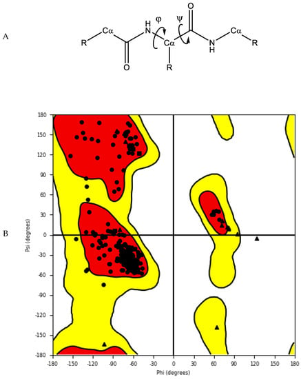
Figure 5. (A) Protein backbone with dihedral angles. (B) An example of a Ramachandran plot of crystal structure of human farnesyl pyrophosphate synthase (PDB ID: 4P0V) [91]. White: disallowed region; yellow: allowed region; red: favourable region.
2.2. Docking-Based Virtual Screening
Docking-based virtual screening aims to discover new drugs by predicting binding modes of both ligand and receptor, studying their interaction patterns, and estimating binding affinity. Some examples of the many docking programs include AutoDock [92], GOLD [93], Glide [94,95], SwissDock [96], DockThor [97], CB-Dock [98] and Molecular Operating Environment (MOE) [99] (Table 1). Due to limitations of X-ray crystallography and NMR spectroscopy, experimentally derived structures often have problems, such as missing hydrogen atoms, incomplete side-chains and loops, ambiguous protonation states and flipped residues. It is therefore essential to prepare the 3D structures accordingly in order to fix these issues before the docking process [100].
The three main goals of molecular docking are: (1) pose prediction to envisage how a ligand may bind to the receptor, (2) virtual screening to search for novel drug candidates from small molecule libraries and (3) binding affinity prediction using scoring functions to estimate the binding affinity of ligands to the receptor [101]. Search algorithms and scoring functions are essential components for molecular docking programs.
A good search algorithm should explore all possible binding modes, and this can be a challenging task. The concept of molecular docking originated from the ‘lock and key’ model proposed by Emil Fischer [102], and early docking programs treated both the protein and ligands as rigid bodies. It was known that protein and ligands are both dynamic entities and that their conformations play an important role in ligand–receptor binding and protein functions, but historically this was too computationally expensive to implement. Modern docking programs treat both protein and ligand with varying degrees of flexibility in order to address this issue.
2.2.1. Binding Site Detection
In docking-based virtual screening, the location of the binding site within the protein must be identified. Most of the protein structures in the PDB are ligand-bound (holo) structures, which defines the binding pocket and provides us with its geometries. In cases where only ligand-free (apo) structures available, there are traditionally three main types of method to identify potential druggable binding sites. Template-based methods such as firestar [103], 3DLigandSite [104] and Libra [105,106] utilise protein sequences to locate residues that are conserved and important for binding. Geometry-based methods, such as CurPocket [98], Surfnet [107] and SiteMap [108,109], search for clefts and pockets based on the size and depths of these cavities. Energy-based methods such as FTMap [110] and Q-SiteFinder [111] locate sites on the surface of a protein that are energetically favourable for binding. Hybrid methods, such as ConCavity [112] and MPLs-Pred [113], as well as machine-learning methods, such as DeepSite [114], Kalasanty [115], and DeepCSeqSite [116] are some of the newer approaches that are under rapid development in recent years.
Beyond locating the orthosteric binding site, these tools are also valuable in identifying potential allosteric binding sites to modulate protein function, hot spots on protein surface to alter protein–protein interactions and also analysing known binding sites to design better molecules that complement the binding pocket. Furthermore, proteins are dynamic systems, and their conformations may change upon ligand binding. Hidden binding pockets, known as cryptic pockets, which are not present in a ligand-free structure, can result from conformational changes upon ligand binding. Detection of cryptic pockets can be a solution to target proteins that were previously considered to be undruggable due to the lack of druggable pockets [117,118].
In addition to the location of the binding site, the evaluation of its potential druggability is equally important. Druggability is the likelihood of being able to modulate a target with a small molecule drug [119]. It can be evaluated on the basis of target information and association, such as protein sequence similarity or genomic information [120]. However, this approach only works for well-studied protein families and homologous proteins may not necessarily bind to structurally similar molecules [121].
Various efforts have been made to evaluate druggability using structure-based approaches. Cheng et al. developed the MAPPOD score, one of the first methods to evaluate druggability, using a physics-based method. MAPPOD model is a binding free energy model combined with curvature and hydrophobic surface area to estimate the maximal achievable affinity for passively absorbed drugs [119]. Halgren developed Dscore, which is a weighted sum of size, enclosure and hydrophobicity [108,109,122]. Other methods to predict druggability include Drug-like Density (DLID) [123], DrugPred [124], DoGSiteScorer [125], FTMap [126] and PockDrug [127].
DoGSiteScorer is a webserver that supports the prediction of potential pockets, characterisation and the druggability estimation. The algorithm first maps a rectangular grid onto the protein; grid points are labelled as either free or occupied depending on whether they lie within the vdW radius of any protein atom. Free grid points are merged to form pockets and subpockets, and neighbouring subpockets are then merged to form pockets. A 3D Difference of Gaussian (DoG) filter is then applied to identify pockets that are favourable to accommodate a ligand. These pockets are characterised global and local descriptors, such as pocket volume, surface, depth, ellipsoidal shape, types of amino acids, presence of metal ions, lipophilic surface, overall hydrophobicity ratio, distances between functional group atoms and many more [125,128].
To predict druggability, a machine learning technique (support vector machine model) trained on a set of known druggable proteins is used to identify druggable pockets based on a subset of these descriptors and to provide a druggability score between 0 to 1, where the higher the score the more druggable is the pocket. A SimpleScore, a linear regression based on size, enclosure and hydrophobicity, is also available to predict druggability [129].
Michel and co-workers used DoGSite, along with FTMap, CryptoSite, as well as SiteMap to predict ligand binding pockets and evaluate druggability of the nucleoside diphosphates attached to sequence-x (NUDIX) hydrolase protein family. Using a dual druggability assessment approach, the authors identified several proteins that are druggable out of the 22 that were studied. This in silico data was also found to correlate well with experimental results [130].
Sitemap locates binding sites by placing ‘site points’ around the protein and each site point is analysed for the proximity to the protein surface and solvent exposure. Site points that fulfil the criteria and are within a given distance of each other are combined into subsites, then subsites that have a relatively small gap between them in a solvent-exposed region are merged to form sites. Distance-field and van der Waals (vdW) grids are then generated to characterise the binding site into three basic regions: hydrophobic, hydrophilic (further separates into H-bond donor, acceptor, and metal-binding region) and neither. Sitemap also evaluates the potential binding sites and computes various properties such as size of the site measured by number of site points, exposure to solvent, degree of enclosure by protein, contact of site points with the protein, hydrophobic and hydrophilic character of the site, and the degree to which a ligand can donate hydrogen bonds. These properties contribute to the calculation of the SiteScore (to distinguish drug-binding and non-drug binding sites) and Dscore (druggability score), which helps to recognise druggable binding sites for virtual screening [108,109].
The transient receptor potential vanilloid 4 (TRPV4) is a widely expressed non-selective cation channel involved in various pathological conditions. Despite the availability of several TRPV4 inhibitors, the binding pocket of TRPV4 and the mechanism of action was not well understood. Doñate-Macian and coworkers used Sitemap to search and assess the binding pocket for one of the known TRPV inhibitors HC067047 based on the crystal structure of Xenopus TRPV4 (Figure 6). This group also further characterised the binding pocket and inhibitor–protein binding interactions with the aid of molecular docking, molecular dynamics and mutagenesis studies. The information was then employed to run a structure-based virtual screening to discover novel TRPV4 inhibitors [131].
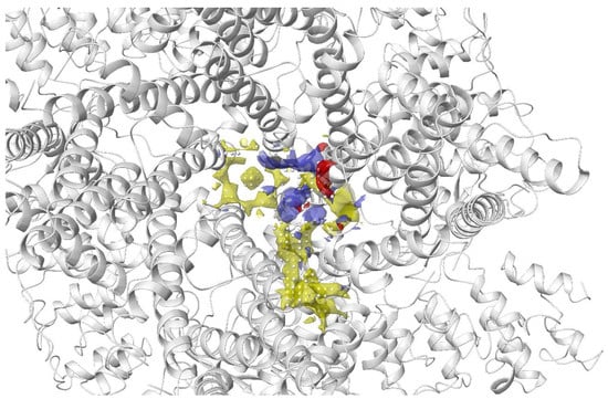
Figure 6. Binding site of TRPV4 detected using Sitemap by Doñate-Macian et al. [131]. Yellow: hydrophobic region; blue: H-bond donor region; red: H-bond acceptor region; white sphere: site point.
2.2.2. Ligand Flexibility
Ligand structures for virtual screening can be obtained from small molecule databases, which are free (e.g., ZINC [132], DrugBank [133] and Pubchem [134]) or commercial (e.g., Maybridge, ChemBridge and Enamine). Conformational sampling of ligands can be performed in several ways. Systematic search generates all possible ligand conformations by exploring all degrees of freedom of the ligand [135]. Carrying out a systematic search using a brute-force approach (exhaustive search) can easily overwhelm the computing power, especially for molecules with many rotatable bonds and therefore rule-based methods have been the more favoured approaches in recent years. Rule-based methods, such as the incremental construction algorithm (also known as anchor and grow method), generate conformations based on known structural preferences of compounds by limiting the conformational space that is being explored. Usually, a knowledge base of allowed torsion angles and ring conformations (e.g., data from the PDB), and possibly a library of 3D fragment conformations, is used to guide the sampling [136,137]. These break the molecule into fragments that are docked into different regions of the receptor. The fragments are then reassembled together to construct a molecule in a low energy conformation.
Conformer generator OMEGA [138] employs a prebuilt library of fragments as well as a knowledge base of torsion angles to generate a large set of conformations, which are sampled by geometric and energy criteria to eliminate conformers with internal clashes. Likewise, ConfGen [139] divides ligands into a core region and peripheral rotamer groups. The core conformation is first generated using a template library, followed by the calculation of the potential energy of rotatable bonds with the torsional term of the OPLS force field, and lastly positioning peripheral groups in their lowest energy forms. To eliminate undesirable conformations or to limit the number of conformations, filtering approaches are applied. Conformations that are too similar are removed based on an energy filter, RMSD, and dihedral angles involving polar hydrogen atoms. Compact conformers are also removed by an empirically derived heuristic scoring method [94,139].
On the other hand, a stochastic search randomly changes the degrees of freedom of the ligand at each step and the change is either accepted or rejected according to a probabilistic criterion such as the Metropolis criterion [140]. Sampling of conformational space can be performed using different techniques in a stochastic search, including Monte Carlo (MC) sampling [62], distance geometry sampling [141] and genetic algorithm-based sampling [142,143]. Balloon [142], a free conformer generator, uses distance geometry to generate an initial conformer for a ligand, followed by a multi-objective genetic algorithm approach to modify torsion angles around rotatable bonds, stereochemistry of double bonds, chiral centres, and ring conformations. Some other tools that were developed for ligand preparation include Prepflow [144], VSPrep [145], Gypsum-DL [146], Frog2 [147] and UNICON [148].
2.2.3. Protein Flexibility
Protein flexibility is essential for their biological function and subtle changes, such as side-chain rearrangements, can alter the size and shape of the binding site and thus bias docking results [149]. Methods to handle protein flexibility can be divided into four groups: soft docking [150,151], side-chain flexibility [152], molecular relaxation [153], and protein ensemble docking [154,155]. Soft docking allows small degrees of overlap between the protein and the ligand by softening the interatomic vdW interactions in docking calculations [151]. These are the simplest methods and are computationally efficient, but they can only account for small changes. Side-chain flexibility allows the sampling of side-chain conformations by varying their essential torsional degrees of freedom, while the protein backbones are kept fixed [156]. The molecular relaxation method involves both protein backbone flexibility and side-chain conformational changes; it first uses rigid-protein docking to place the ligand into the binding site then relaxes the protein backbone and the nearby side-chain atoms, usually employing methods, such as MC and MD [157,158,159]. Protein ensemble docking methods dock the ligand on a set of rigid protein structures, with different conformations which represent a flexible receptor. The docking results for each conformation are then re-analysed [160].
Most contemporary docking approaches treat proteins with partial or complete flexibility. For instance, Schrödinger offers a range of docking methodologies with different treatment of protein flexibility. Glide [94,95], with standard precision (SP) and extra precision (XP) is a docking strategy, which allows conformational flexibility for the ligands but treats the receptor as a rigid entity. It softens the active site via vdW scaling (soft docking) with the option of rotamer configuration sampling. Meanwhile, a superior method, Induced Fit Docking, uses Glide for docking to account for ligand flexibility, and Prime [161,162] for side-chain optimisation to account for receptor flexibility [163]. The ligand is docked into the receptor using Glide with vdW scaling and flexible side-chains are temporarily mutated to alanine to reduce steric clashes and the blocking of the binding site. Once the docking poses are generated, the mutated residues are restored to their original residues and Prime (a program for protein structure predictions) [161,162] is used to predict and reorient the side-chains with each ligand pose. The ligand–receptor complex is then minimised to afford a low-energy protein conformation, which is used for ligand resampling with Glide.
Water molecules have a crucial role in biological systems and interactions, such as stabilising protein–ligand complex, biomolecular recognition and participating in H-bond networks. Water molecules can participate in ligand–protein interactions by acting as bridging waters, and their displacement from the binding site upon ligand binding can also contribute to binding affinity, playing a significant role in the thermodynamics of protein-ligand binding [164]. The retention or removal of water molecules during virtual screening can have a direct impact on the size, shape and chemical properties of the binding site, which can influence binding geometries and affinity calculations.
Due to the ability of a water molecule to act as both an H-bond donor and acceptor, as well as its highly mobile nature, predicting the location and contribution of water molecules in protein–ligand binding is a challenging task. Crystal structures or cryo-EM structures of proteins can sometimes capture the placement of water molecules in the protein matrix, but the information is not always accurate due to the low resolution of the structural data, and the sample preparation conditions do not reflect the biological environment [165,166,167,168].
Many approaches were developed to simulate and predict the behaviour of water molecules. Implicit models, also known as continuum models, treat water molecules as a uniform and continuous medium. The free energy of solvation is traditionally estimated based on three parameters, the free energy required to form the solute cavity, vdW interactions and electrostatic interactions between solute and solvent. This method is less computationally demanding but neglects details at the solute–solvent interface [167,168]. Explicit models are computationally more expensive, but the molecular details of each water molecule are considered. Water molecules are normally described using a three-, four-, or five-point model.
In protein–ligand docking, water can be treated explicitly or in an approach involving a combination of implicit and explicit (hybrid), and they can be separated into four categories: (1) Empirical and knowledge-based methods (e.g., Consolv [169] and WaterScore [170]), (2) statistical and molecular mechanics methods (e.g., GRID [171,172], 3D-RISM [173,174], SZMAP [175]), (3) MD simulation methods (e.g., WaterMap [176], GIST [177], SPAM [116]) and, lastly, (4) Monte Carlo simulation methods (e.g., JAWS [178]).
2.2.4. Scoring Functions
After searching for all possible binding modes, a scoring function is used to evaluate the quality of the docking poses. Scoring functions determine the binding mode and estimate binding affinity, which assists in identifying and ranking potential drug candidates. There are three main categories of scoring functions: force field-based, empirical-based, and knowledge-based methods.
Force field-based scoring functions generally use standard force field parameters taken from force fields, such as AMBER [179], which consider both the intramolecular energy of the ligand and the intermolecular energy of the protein–ligand complex [180]. The ΔG estimated using this scoring function is the sum of these energies, which is generally composed of vdW and electrostatic energy terms. An example of program that uses this method is DOCK, which utilises the following equation: [181,182]
where rij is the distance between protein atom i and ligand atom j, Aij and Bij are vdW components (repulsive and attractive vdW), qi and qj are atomic charges and ε(rij) is the distance-dependent dielectric constant.
Empirical-based functions estimate binding affinity based upon a set of weighted energy terms that are described in the following equation:
The energy terms (ΔGi) represents energy terms such as vdW energy, electrostatic energy, hydrogen (H) bond interactions, desolvation, entropy, hydrophobicity, etc., whereas the weighting factors (Wi) are determined via regression analysis by fitting the binding affinity data of a training set of protein–ligand complex with known 3D structures [94]. The first empirical scoring function (SCORE) was developed by Böhm in 1994 [183] based upon a dataset of 45 protein–ligand complexes, and the scoring function considers four energy terms: hydrogen bonds, ionic interactions, the lipophilic protein–ligand contact surface and the number of rotatable bonds in the ligand. Over time, the empirical scoring function has evolved by expanding the data set and considering more energy terms. For example, ChemScore, developed by Eldridge et al. [184], also considers metal atoms contribution and Glide XP score includes terms to account for desolvation effects [94].
In knowledge-based functions, structural information is extracted from experimentally determined structures of protein–ligand complexes from databases, such as the PDB [30] and Cambridge Structural Database (CSD) [185,186]. Boltzmann law is employed to transform the protein–ligand atom pair preferences into distance-dependent pairwise potentials, and the favourability of the binding modes of atom pairs is related to the frequency observed in known protein–ligand structures [187,188]. The potentials are calculated using the following equation:
where w(r) is the pairwise potential between protein and ligand, KB is the Boltzmann constant, T is the absolute temperature of the system, ρ(r) is the number density of the protein–ligand atom pair at distance r, and ρ∗(r) is the pair density in a reference state where the interatomic interactions are zero.
Table 1. List of common docking programs.
| Program | Ligand Flexibility | Receptor Flexibility | Scoring Functions | Examples of Application |
|---|---|---|---|---|
| Glide (HTVS, SP and XP) [94,95,189] | Exhaustive ligand conformation search | Soft docking | Empirical | Discovery of novel fibroblast growth factor receptor 1 kinase inhibitors [190] and CDK5 inhibitors [191] |
| GOLD [93] | Genetic algorithm | Soft docking Ensemble docking Side-chain flexibility |
Goldscore (empirical) Chemscore (empirical) ChemPLP (empirical) ASP (knowledge based) |
Design of non-peptide MDM2 inhibitors [192] |
| Autodock 4 [193] | Genetic Algorithm Simulated Annealing Local Search Lamarckian Genetic Algorithm |
Side-chain flexibility | Semi-empirical free energy force field | Discovery of reversible NEDD8 activating enzyme inhibitor [194] |
| DOCK 6 [195] | Incremental construction algorithm | Rigid | Force field | Design and development of potent and selective dual BRD4/PLK1 Inhibitors [196] |
| Internal Coordinates Mechanics (ICM) [197] | Stochastic search (MC) | Side-chain flexibility (rotamer libraries) | Force field | Discovery of novel retinoic acid receptor agonist [198] and enoyl-acyl carrier protein reductase inhibitors in Plasmodium falciparum [199] |
| Surflex [200,201] | Incremental construction algorithm | Ensemble docking | Empirical | Discovery of novel inhibitors of Leishmania donovani γ-glutamylcysteine synthetase [202] |
| MOE [99,203,204,205] | Systematic (exhaustive) Stochastic High throughput Conformational Import (incremental construction + stochastic) [99] |
Rigid | ASE (empirical) Affinity dG (empirical) Alpha HB (empirical) GBVI/WSA (force field) |
Identification of novel monoamine oxidase B inhibitors [206] and Chk1 inhibitors [207] |
| FlexX [208,209] | Incremental construction algorithm | Rigid | Empirical | Identification of PKB inhibitors [210] and phosphodiesterase 4 inhibitors [211] |
| FRED [212,213] | Systematic (exhaustive) search, precomputed using Omega (using torsion and ring libraries) [138] | Rigid | Chemgauss 3 (empirical) Chemgauss 4 (empirical) |
Discovery of selective butyrylcholinesterase inhibitors [214] |
Abbreviations: ASP: Astex Statistical Potential; BRD4: Bromodomain 4; CDK5: Cyclin dependent kinase 5; ChemPLP: Piecewise Linear Potential; HTVS: high throughput virtual screening; MDM2: Mouse double minute 2 homolog; PKB: Protein kinase B; PLK1: Polo-like Kinase 1.
This entry is adapted from the peer-reviewed paper 10.3390/pharmaceutics15010049
This entry is offline, you can click here to edit this entry!