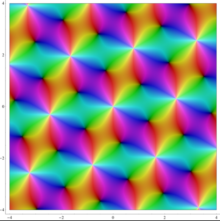
In mathematics, Weierstrass's elliptic functions are elliptic functions that take a particularly simple form. They are named for Karl Weierstrass. This class of functions are also referred to as p-functions and they are usually denoted by the symbol ℘. They play an important role in theory of elliptic functions. A ℘-function together with its derivative can be used to parameterize elliptic curves and they generate the field of elliptic functions with respect to a given period lattice.
- elliptic functions
- elliptic curves
- ℘-function
1. Definition
Let [math]\displaystyle{ \omega_1,\omega_2\in\mathbb{C} }[/math] be two complex numbers that are linear independent over [math]\displaystyle{ \mathbb{R} }[/math] and let [math]\displaystyle{ \Lambda:=\mathbb{Z}\omega_1+\mathbb{Z}\omega_2:=\{m\omega_1+n\omega_2: m,n\in\mathbb{Z}\} }[/math] be the lattice generated by those numbers. Then the [math]\displaystyle{ \wp }[/math]-function is defined as follows:
- [math]\displaystyle{ \weierp(z,\omega_1,\omega_2):=\weierp(z,\Lambda) := \frac{1}{z^2} + \sum_{\lambda\in\Lambda\setminus\{0\}}\left(\frac 1 {(z-\lambda)^2} - \frac 1 {\lambda^2}\right). }[/math]
This series converges locally uniformly absolutely in [math]\displaystyle{ \mathbb{C}\setminus\Lambda }[/math]. Oftentimes instead of [math]\displaystyle{ \wp(z,\omega_1,\omega_2) }[/math] only [math]\displaystyle{ \wp(z) }[/math] is written.
The Weierstrass [math]\displaystyle{ \wp }[/math]-function is constructed exactly in such a way that it has a pole of the order two at each lattice point.
Because the sum [math]\displaystyle{ \sum_{\lambda\in\Lambda}\frac 1{(z-\lambda)^2} }[/math] alone would not converge it is necessary to add the term [math]\displaystyle{ -\frac 1 {\lambda^2} }[/math].[1]
It is common to use [math]\displaystyle{ 1 }[/math] and [math]\displaystyle{ \tau\in\mathbb{H}:=\{z\in\mathbb{C}:\operatorname{Im}(z)\gt 0\} }[/math] as generators of the lattice. Multiplying by [math]\displaystyle{ \frac 1{\omega_1} }[/math] maps the lattice [math]\displaystyle{ \mathbb{Z}\omega_1+\mathbb{Z}\omega_2 }[/math] isomorphically onto the lattice [math]\displaystyle{ \mathbb{Z}+\mathbb{Z}\tau }[/math] with [math]\displaystyle{ \tau=\frac{\omega_2}{\omega_1} }[/math]. By possibly substituting [math]\displaystyle{ \tau }[/math] by [math]\displaystyle{ -\tau }[/math] it can be assumed that [math]\displaystyle{ \tau\in\mathbb{H} }[/math]. One sets [math]\displaystyle{ \wp(z,\tau) := \wp(z, 1,\tau) }[/math].
2. Motivation
A cubic of the form [math]\displaystyle{ C_{g_2,g_3}^\mathbb{C}=\{(x,y)\in\mathbb{C}^2:y^2=4x^3-g_2x+g_3\} }[/math], where [math]\displaystyle{ g_2,g_3\in\mathbb{C} }[/math] are complex numbers with [math]\displaystyle{ g_2^3-27g_3^2\neq0 }[/math], can not be rationally parameterized.[2] Yet one still wants to find a way to parameterize it.
For the quadric [math]\displaystyle{ K=\{(x,y)\in\mathbb{R}^2:x^2+y^2=1\} }[/math], the unit circle, there exists a (non-rational) parameterization using the sine function and its derivative the cosine function:
- [math]\displaystyle{ \psi:\mathbb{R}/2\pi\mathbb{Z}\to K, \quad t\mapsto(\sin(t),\cos(t)) }[/math].
Because of the periodicity of the sine and cosine [math]\displaystyle{ \mathbb{R}/2\pi\mathbb{Z} }[/math] is chosen to be the domain, so the function is bijective.
In a similar way one can get a parameterization of [math]\displaystyle{ C_{g_2,g_3}^\mathbb{C} }[/math] by means of the doubly periodic [math]\displaystyle{ \wp }[/math]-function (see in the section "Relation to ellitpic curves"). This parameterization has the domain [math]\displaystyle{ \mathbb{C}/\Lambda }[/math], which is topologically equivalent to a torus.[3]
There is another analogy to the trigonometric functions. Consider the integral function
- [math]\displaystyle{ a(x)=\int_0^x\frac{dy}{\sqrt{(1-y^2)}} }[/math].
It can be simplified by substituting [math]\displaystyle{ y=\sin(t) }[/math] and [math]\displaystyle{ s=\arcsin(x) }[/math]:
- [math]\displaystyle{ a(x)=\int_0^sdt=s=\arcsin(x) }[/math].
That means [math]\displaystyle{ a^{-1}(x)=\sin(x) }[/math]. So the sine function is an inverse function of an integral function.[4]
Elliptic functions are also inverse functions of integral functions, namely of elliptic integrals. In particular the [math]\displaystyle{ \wp }[/math]-function is obtained in the following way:
Let
- [math]\displaystyle{ u(z)=-\int_z^\infin\frac{ds}{\sqrt{4s^3-g_2s-g_3}} }[/math].
Then [math]\displaystyle{ u^{-1} }[/math] can be extended to the complex plane and this extension equals the [math]\displaystyle{ \wp }[/math]-function.[5]
3. Properties
- ℘ is an even function. That means [math]\displaystyle{ \wp(z)=\wp(-z) }[/math] for all [math]\displaystyle{ z \in \mathbb{C} \setminus \Lambda }[/math], which can be seen in the following way:
- [math]\displaystyle{ \weierp(-z)=\frac{1}{(-z)^2}+\sum_{\lambda\in\Lambda\setminus\{0\}}\left(\frac1{(-z-\lambda)^2}-\frac1{\lambda^2}\right)=\frac{1}{z^2}+\sum_{\lambda\in\Lambda\setminus\{0\}}\left(\frac1{(z+\lambda)^2}-\frac1{\lambda^2}\right)=\frac{1}{z^2}+\sum_{\lambda\in\Lambda\setminus\{0\}}\left(\frac1{(z-\lambda)^2}-\frac1{\lambda^2}\right)=\wp(z) }[/math]
The second last equality holds because [math]\displaystyle{ \{-\lambda:\lambda \in \Lambda\}=\Lambda }[/math]. Since the sum converges absolutely this rearrangement does not change the limit.
- ℘ is meromorphic and its derivative is[6]
- [math]\displaystyle{ \wp'(z)=-2\sum_{\lambda \in \Lambda}\frac1{(z-\lambda)^3} }[/math].
- [math]\displaystyle{ \wp }[/math] and [math]\displaystyle{ \wp' }[/math] are doubly periodic with the periods [math]\displaystyle{ \omega_1 }[/math]und [math]\displaystyle{ \omega_2 }[/math].[6] This means:
- [math]\displaystyle{ \wp(z+\omega_1)=\wp(z)=\wp(z+\omega_2) }[/math] and [math]\displaystyle{ \wp'(z+\omega_1)=\wp'(z)=\wp'(z+\omega_2) }[/math].
It follows that [math]\displaystyle{ \wp(z+\lambda)=\wp(z) }[/math] and [math]\displaystyle{ \wp'(z+\lambda)=\wp'(z) }[/math] for all [math]\displaystyle{ \lambda \in \Lambda }[/math]. Functions which are meromorphic and doubly periodic are also called elliptic functions.
4. Laurent Expansion
Let [math]\displaystyle{ r:=\min\{{|\lambda}|:0\neq\lambda\in\Lambda\} }[/math]. Then for [math]\displaystyle{ 0\lt |z|\lt r }[/math] the [math]\displaystyle{ \wp }[/math]-function has the following Laurent expansion
- [math]\displaystyle{ \wp(z)=\frac1{z^2}+\sum_{n=1}^\infin (2n+1)G_{2n+2}z^{2n} }[/math]
where
- [math]\displaystyle{ G_n=\sum_{0\neq\lambda\in\Lambda}\lambda^{-n} }[/math] for [math]\displaystyle{ n\geq3 }[/math] are so called Eisenstein series.[6]
5. Differential Equation
Set [math]\displaystyle{ g_2=60G_4 }[/math] and [math]\displaystyle{ g_3=140G_6 }[/math]. Then the [math]\displaystyle{ \wp }[/math]-function satisfies the differential equation[6]
- [math]\displaystyle{ \wp'^2(z) = 4\wp ^3(z)-g_2\wp(z)-g_3 }[/math].
This relation can be verified by forming a linear combination of powers of [math]\displaystyle{ \wp }[/math] and [math]\displaystyle{ \wp' }[/math] to eliminate the pole at [math]\displaystyle{ z=0 }[/math]. This yields an entire elliptic function that has to be constant by Liouville's theorem .[6]
6. Invariants
The coefficients of the above differential equation g2 and g3 are known as the invariants. Because they depent on the lattice [math]\displaystyle{ \Lambda }[/math] they can be viewed as functions in [math]\displaystyle{ \omega_1 }[/math]and [math]\displaystyle{ \omega_2 }[/math].
The series expansion suggests that g2 and g3 are homogeneous functions of degree −4 and −6. That is[7]
- [math]\displaystyle{ g_2(\lambda \omega_1, \lambda \omega_2) = \lambda^{-4} g_2(\omega_1, \omega_2) }[/math]
- [math]\displaystyle{ g_3(\lambda \omega_1, \lambda \omega_2) = \lambda^{-6} g_3(\omega_1, \omega_2) }[/math] for [math]\displaystyle{ \lambda\neq0 }[/math].
If [math]\displaystyle{ \omega_1 }[/math]and [math]\displaystyle{ \omega_2 }[/math] are chosen in such a way that [math]\displaystyle{ \operatorname{Im}\left( \frac{\omega_2}{\omega_1} \right)\gt 0 }[/math] g2 and g3 can be interpreted as functions on the upper half-plane [math]\displaystyle{ \mathbb{H}:=\{z\in\mathbb{C}:\operatorname{Im}(z)\gt 0\} }[/math].
Let [math]\displaystyle{ \tau=\frac{\omega_2}{\omega_1} }[/math]. One has:[8]
- [math]\displaystyle{ g_2(1,\tau)=\omega_1^4g_2(\omega_1,\omega_2) }[/math],
- [math]\displaystyle{ g_3(1,\tau)=\omega_1^6 g_3(\omega_1,\omega_2) }[/math].
That means g2 and g3 are only scaled by doing this. Set
[math]\displaystyle{ g_2(\tau):=g_2(1,\tau) }[/math], [math]\displaystyle{ g_3(\tau):=g_3(1,\tau) }[/math].
As functions of [math]\displaystyle{ \tau\in\mathbb{H} }[/math] [math]\displaystyle{ g_2,g_3 }[/math] are so called modular forms.
The Fourier series for [math]\displaystyle{ g_2 }[/math] and [math]\displaystyle{ g_3 }[/math] are given as follows:[9]
- [math]\displaystyle{ g_2(\tau)=\frac{4}{3}\pi^4 \left[ 1+ 240\sum_{k=1}^\infty \sigma_3(k) q^{2k} \right] }[/math]
- [math]\displaystyle{ g_3(\tau)=\frac{8}{27}\pi^6 \left[ 1- 504\sum_{k=1}^\infty \sigma_5(k) q^{2k} \right] }[/math]
where [math]\displaystyle{ \sigma_a(k):=\sum_{d\mid{k}}d^\alpha }[/math] is the divisor function and [math]\displaystyle{ q:=\exp(i\pi\tau) }[/math].
7. Modular Discriminant
The modular discriminant Δ is defined as the discriminant of the polynomial at right-hand side of the above differential equation:
- [math]\displaystyle{ \Delta=g_2^3-27g_3^2. \, }[/math]
The discriminant is a modular form of weight 12. That is, under the action of the modular group, it transforms as
- [math]\displaystyle{ \Delta \left( \frac {a\tau+b} {c\tau+d}\right) = \left(c\tau+d\right)^{12} \Delta(\tau) }[/math]
where [math]\displaystyle{ a,b,d,c\in\mathbb{Z} }[/math] with ad − bc = 1.[10]
Note that [math]\displaystyle{ \Delta=(2\pi)^{12}\eta^{24} }[/math] where [math]\displaystyle{ \eta }[/math] is the Dedekind eta function.[11]
For the Fourier coefficients of [math]\displaystyle{ \Delta }[/math], see Ramanujan tau function.
8. The Constants e1, e2 and e3
[math]\displaystyle{ e_1 }[/math], [math]\displaystyle{ e_2 }[/math] and [math]\displaystyle{ e_3 }[/math] are usually used to denote the values of the [math]\displaystyle{ \wp }[/math]-function at the half-periods.
- [math]\displaystyle{ e_1\equiv\wp\left(\frac{\omega_1}{2}\right) }[/math]
- [math]\displaystyle{ e_2\equiv\wp\left(\frac{\omega_2}{2}\right) }[/math]
- [math]\displaystyle{ e_3\equiv\wp\left(\frac{\omega_1+\omega_2}{2}\right) }[/math]
They are pairwise distinct and only depend on the lattice [math]\displaystyle{ \Lambda }[/math] and not on its generators.[12]
[math]\displaystyle{ e_1 }[/math], [math]\displaystyle{ e_2 }[/math] and [math]\displaystyle{ e_3 }[/math] are the roots of the cubic polynomial [math]\displaystyle{ 4\wp(z)^3-g_2\wp(z)-g_3 }[/math] and are related by the equation:
- [math]\displaystyle{ e_1+e_2+e_3=0 }[/math].
Because those roots are distinct the discriminant [math]\displaystyle{ \Delta }[/math] does not vanish on the upper half plane.[13] Now we can rewrite the differential equation:
- [math]\displaystyle{ \wp'^2(z)=4(\wp(z)-e_1)(\wp(z)-e_2)(\wp(z)-e_3) }[/math].
That means the half-periods are zeros of [math]\displaystyle{ \wp' }[/math].
The invariants [math]\displaystyle{ g_2 }[/math] and [math]\displaystyle{ g_3 }[/math] can be expressed in terms of these constants in the following way:[14]
- [math]\displaystyle{ g_2=-4(e_1e_2+e_1e_3+e_2e_3) }[/math]
- [math]\displaystyle{ g_3=4e_1e_2e_3 }[/math]
9. Relation to Elliptic Curves
Consider the projective cubic curve
- [math]\displaystyle{ \bar C_{g_2,g_3}^\mathbb{C}=\{(x,y)\in\mathbb{C}^2:y^2=4x^3-g_2x+g_3\}\cup\{\infin\}\subset\mathbb{P}_\mathbb{C}^2 }[/math].
For this cubic, also called Weierstrass cubic, there exists no rational parameterization, if [math]\displaystyle{ \Delta\neq0 }[/math].[2] In this case it is also called an elliptic curve. Nevertheless there is a parameterization that uses the [math]\displaystyle{ \wp }[/math]-function and its derivative [math]\displaystyle{ \wp' }[/math]:[15]
[math]\displaystyle{ \varphi: \mathbb{C}/\Lambda\to\bar C_{g_2,g_3}^\mathbb{C}, \quad \bar{z}\mapsto \begin{cases} (\wp(z),\wp'(z),1) & \bar{z}\neq0\\ \infin \quad &\bar{z}=0 \end{cases} }[/math]
Now the map [math]\displaystyle{ \varphi }[/math] is bijective and parameterizes the elliptic curve [math]\displaystyle{ \bar C_{g_2,g_3}^\mathbb{C} }[/math].
[math]\displaystyle{ \mathbb{C}/\Lambda }[/math] is an abelian group and a topological space, equipped with the quotient topology.
It can be shown that every Weierstrass cubic is given in such a way. That is to say that for every pair [math]\displaystyle{ g_2,g_3\in\mathbb{C} }[/math] with [math]\displaystyle{ \Delta=g_2^3-27g_3^2\neq0 }[/math] there exists a lattice [math]\displaystyle{ \mathbb{Z}\omega_1+\mathbb{Z}\omega_2 }[/math], such that
[math]\displaystyle{ g_2=g_2(\omega_1,\omega_2) }[/math] and [math]\displaystyle{ g_3=g_3(\omega_1,\omega_2) }[/math].[16]
The statement that elliptic curves over [math]\displaystyle{ \mathbb{Q} }[/math] can be parameterized over [math]\displaystyle{ \mathbb{Q} }[/math], is known as the modularity theorem. This is an important theorem in number theory. It was part of Andrew Wiles' proof (1995) of Fermat's Last Theorem.
10. Addition Theorems
Let [math]\displaystyle{ z,w\in\mathbb{C} }[/math], so that [math]\displaystyle{ z,w,z+w,z-w\notin\Lambda }[/math]. Then one has:[17]
- [math]\displaystyle{ \wp(z+w)=\frac1{4} \left[\frac{\wp'(z)-\wp'(w)}{\wp(z)-\wp(w)}\right]^2-\wp(z)-\wp(w) }[/math].
As well as the duplication formula:[17]
-
- [math]\displaystyle{ \wp(2z)=\frac1{4}\left[\frac{\wp''(z)}{\wp'(z)}\right]^2-2\wp(z) }[/math].
These formulas also have a geometric interpretation, if one looks at the elliptic curve [math]\displaystyle{ \bar C_{g_2,g_3}^\mathbb{C} }[/math] together with the mapping [math]\displaystyle{ {\varphi}:\mathbb{C}/\Lambda\to\bar C_{g_2,g_3}^\mathbb{C} }[/math] as in the previous section.
The group structure of [math]\displaystyle{ (\mathbb{C}/\Lambda,+) }[/math] translates to the curve [math]\displaystyle{ \bar C_{g_2,g_3}^\mathbb{C} }[/math]and can be geometrically interpreted there:
The sum of three pairwise different points [math]\displaystyle{ a,b,c\in\bar C_{g_2,g_3}^\mathbb{C} }[/math]is zero if and only if they lie on the same line in [math]\displaystyle{ \mathbb{P}_\mathbb{C}^2 }[/math].[18]
This is equivalent to:
- [math]\displaystyle{ \det\left(\begin{array}{rrr} 1&\wp(u+v)&-\wp'(u+v)\\ 1&\wp(v)&\wp'(v)\\ 1&\wp(u)&\wp'(u)\\ \end{array}\right) =0 }[/math],
where [math]\displaystyle{ \wp(u)=a }[/math], [math]\displaystyle{ \wp(v)=b }[/math] and [math]\displaystyle{ u,v\notin\Lambda }[/math].[19]
11. Relation to Jacobi's Elliptic Functions
For numerical work, it is often convenient to calculate the Weierstrass elliptic function in terms of Jacobi's elliptic functions.
The basic relations are:[20]
- [math]\displaystyle{ \wp(z) = e_3 + \frac{e_1 - e_3}{\operatorname{sn}^2 w} = e_2 + ( e_1 - e_3 ) \frac{\operatorname{dn}^2 w}{\operatorname{sn}^2 w} = e_1 + ( e_1 - e_3 ) \frac{\operatorname{cn}^2 w}{\operatorname{sn}^2 w} }[/math]
where [math]\displaystyle{ e_1,e_2 }[/math]and [math]\displaystyle{ e_3 }[/math] are the three roots described above and where the modulus k of the Jacobi functions equals
- [math]\displaystyle{ k =\sqrt{\frac{e_2 - e_3}{e_1 - e_3}} }[/math]
and their argument w equals
- [math]\displaystyle{ w =z \sqrt{e_1 - e_3}. }[/math]
12. Typography
The Weierstrass's elliptic function is usually written with a rather special, lower case script letter ℘.[21]
In computing, the letter ℘ is available as \wp in TeX. In Unicode the code point is U+2118 ℘ SCRIPT CAPITAL P (HTML ℘ · ℘), with the more correct alias weierstrass elliptic function.[22] In HTML, it can be escaped as ℘.
| Preview | Template:Charmap/showcharTemplate:Charmap/showcharTemplate:Charmap/showcharTemplate:Charmap/showchar | |
|---|---|---|
| Unicode name | SCRIPT CAPITAL P / WEIERSTRASS ELLIPTIC FUNCTION | |
| Encodings | decimal | hex |
| Unicode | 8472 0 0 0 | U+2118 |
| UTF-8 | 226 132 152 0 0 0 | E2 84 98 00 00 00 |
| Numeric character reference | ℘ |
℘ |
| Named character reference | ℘ | |
The content is sourced from: https://handwiki.org/wiki/Weierstrass%27s_elliptic_functions
References
- Apostol, Tom M. (1976). Modular functions and Dirichlet series in number theory. New York: Springer-Verlag. pp. 9. ISBN 0-387-90185-X. OCLC 2121639. https://www.worldcat.org/oclc/2121639.
- Hulek, Klaus. (2012) (in German), Elementare Algebraische Geometrie : Grundlegende Begriffe und Techniken mit zahlreichen Beispielen und Anwendungen (2., überarb. u. erw. Aufl. 2012 ed.), Wiesbaden: Vieweg+Teubner Verlag, p. 8, ISBN 978-3-8348-2348-9
- Rolf Busam (2006) (in German), Funktionentheorie 1 (4., korr. und erw. Aufl ed.), Berlin: Springer, p. 259, ISBN 978-3-540-32058-6
- Jeremy Gray (2015) (in German), Real and the complex : a history of analysis in the 19th century, Cham, p. 71, ISBN 978-3-319-23715-2
- Rolf Busam (2006) (in German), Funktionentheorie 1 (4., korr. und erw. Aufl ed.), Berlin: Springer, p. 294, ISBN 978-3-540-32058-6
- Apostol, Tom M. (1976) (in German), Modular functions and Dirichlet series in number theory, New York: Springer-Verlag, p. 11, ISBN 0-387-90185-X
- Apostol, Tom M. (1976). Modular functions and Dirichlet series in number theory. New York: Springer-Verlag. pp. 14. ISBN 0-387-90185-X. OCLC 2121639. https://www.worldcat.org/oclc/2121639.
- Apostol, Tom M. (1976) (in German), Modular functions and Dirichlet series in number theory, New York: Springer-Verlag, p. 14, ISBN 0-387-90185-X
- Apostol, Tom M. (1990). Modular functions and Dirichlet series in number theory (2nd ed.). New York: Springer-Verlag. pp. 20. ISBN 0-387-97127-0. OCLC 20262861. https://www.worldcat.org/oclc/20262861.
- Apostol, Tom M. (1976). Modular functions and Dirichlet series in number theory. New York: Springer-Verlag. pp. 50. ISBN 0-387-90185-X. OCLC 2121639. https://www.worldcat.org/oclc/2121639.
- Chandrasekharan, K. (Komaravolu), 1920- (1985). Elliptic functions. Berlin: Springer-Verlag. pp. 122. ISBN 0-387-15295-4. OCLC 12053023. https://www.worldcat.org/oclc/12053023.
- Rolf Busam (2006) (in German), Funktionentheorie 1 (4., korr. und erw. Aufl ed.), Berlin: Springer, p. 270, ISBN 978-3-540-32058-6
- Tom M. Apostol (1976) (in German), Modular functions and Dirichlet series in number theory, New York: Springer-Verlag, p. 13, ISBN 0-387-90185-X
- K. Chandrasekharan (1985) (in German), Elliptic functions, Berlin: Springer-Verlag, p. 33, ISBN 0-387-15295-4
- Hulek, Klaus. (2012) (in German), Elementare Algebraische Geometrie : Grundlegende Begriffe und Techniken mit zahlreichen Beispielen und Anwendungen (2., überarb. u. erw. Aufl. 2012 ed.), Wiesbaden: Vieweg+Teubner Verlag, p. 12, ISBN 978-3-8348-2348-9
- Hulek, Klaus. (2012) (in German), Elementare Algebraische Geometrie : Grundlegende Begriffe und Techniken mit zahlreichen Beispielen und Anwendungen (2., überarb. u. erw. Aufl. 2012 ed.), Wiesbaden: Vieweg+Teubner Verlag, p. 111, ISBN 978-3-8348-2348-9
- Rolf Busam (2006) (in German), Funktionentheorie 1 (4., korr. und erw. Aufl ed.), Berlin: Springer, p. 286, ISBN 978-3-540-32058-6
- Rolf Busam (2006) (in German), Funktionentheorie 1 (4., korr. und erw. Aufl ed.), Berlin: Springer, p. 287, ISBN 978-3-540-32058-6
- Rolf Busam (2006) (in German), Funktionentheorie 1 (4., korr. und erw. Aufl ed.), Berlin: Springer, p. 288, ISBN 978-3-540-32058-6
- Korn GA, Korn TM (1961). Mathematical Handbook for Scientists and Engineers. New York: McGraw–Hill. pp. 721.
- This symbol was used already at least in 1890. The first edition of A Course of Modern Analysis by E. T. Whittaker in 1902 also used it.[21]
- The Unicode Consortium has acknowledged two problems with the letter's name: the letter is in fact lowercase, and it is not a "script" class letter, like U+1D4C5 𝓅 MATHEMATICAL SCRIPT SMALL P, but the letter for Weierstrass's elliptic function. Unicode added the alias as a correction.[22][23]