Abstract: In the past, the Lorenz 1963 and 1969 models ^[1][2]have been applied for revealing the chaotic nature of weather and climate and for estimating the atmospheric predictability limit. Recently, an in-depth analysis of classical Lorenz 1963 models and newly developed, generalized Lorenz models suggested a revised view that “the entirety of weather possesses a dual nature of chaos and order with distinct predictability”,^[3][4][5] in contrast to the conventional view of “weather is chaotic”. The distinct predictability associated with attractor coexistence suggests limited predictability for chaotic solutions and unlimited predictability (or up to their lifetime) for non-chaotic solutions. Such a view is also supported by a recent analysis of the Lorenz 1969 model that is capable of producing both unstable and stable solutions.^[6] While the alternative appearance of two kinds of attractor coexistence was previously illustrated, in this study, multistability (for attractor coexistence) and monostability (for single-type solutions) are further discussed using kayaking and skiing as an analogy. Using a slowly varying, periodic heating parameter, we additionally emphasize the predictable nature of recurrence for slowly varying solutions and a less predictable (or unpredictable) nature for the onset for emerging solutions (defined as the exact timing for the transition from a chaotic solution to a non-chaotic limit cycle type solution). As a result, we refined the revised view outlined above to: “The atmosphere possesses chaos and order; it includes, as examples, emerging organized systems (such as tornadoes) and time-varying forcing from recurrent seasons”. In addition to diurnal and annual cycles, examples of non-chaotic weather systems, as previously documented, are provided to support the revised view.

An Analogy for Monostability and Multistability Using Skiing and Kayaking

Since the sensitive dependence of solutions on initial conditions (SDIC), monostability, and multistability are the most important concepts in this study, to help readers, they are first illustrated using real-world analogies of skiing and kayaking. To explain SDIC, the book entitled “The Essence of Chaos” by Lorenz ^[7], 1993 applied the activity of skiing (left in Figure 1) and developed an idealized skiing model for revealing the sensitivity of time-varying paths to initial positions (middle in Figure 1). Based on the left panel, when slopes are steep everywhere, SDIC always appears. This feature with a single type of solution is referred to as monostability. 

In comparison, the right panel of Figure 1 for kayaking is used to illustrate multistability. In the photo, the appearance of strong currents and a stagnant area (outlined with a white box) suggests instability and local stability, respectively. As a result, when two kayaks move along strong currents, their paths display SDIC. On the other hand, when two kayaks move into a stagnant area, they become trapped, showing no typical SDIC (although a chaotic transient may occur^[8]). Such features of SDIC or no SDIC suggest two types of solutions and illustrate the nature of multistability.

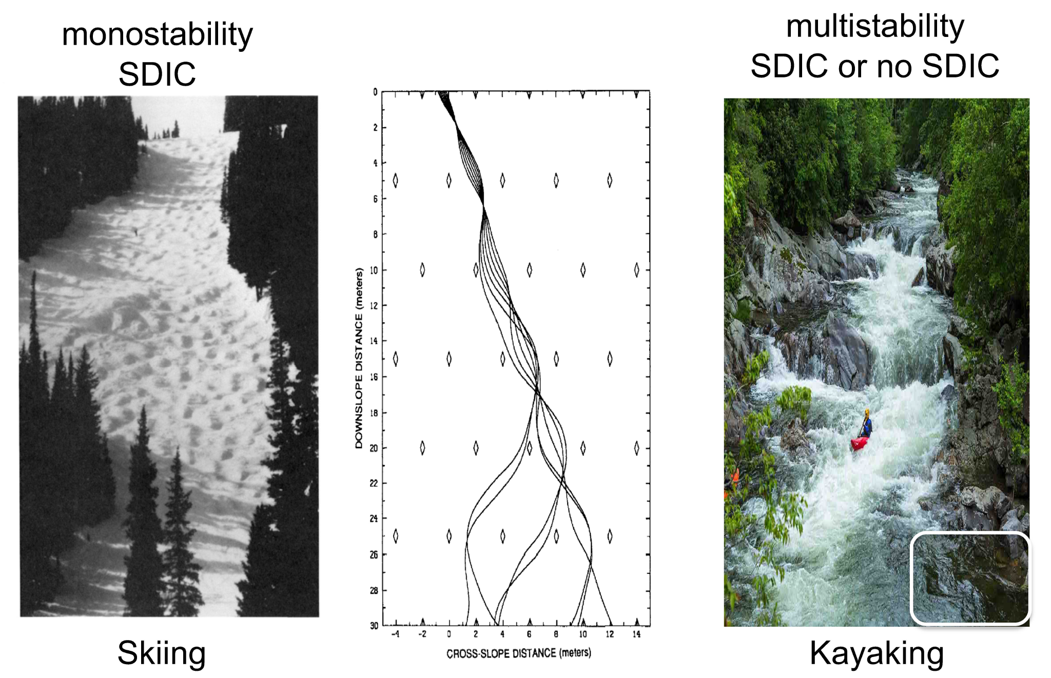
Figure 1. Skiing as used to reveal monostability (left and middle, Lorenz 1993 [3]) and kayaking as used to indicate multistability (right, courtesy of Shutterstock-Carol Mellema  https://www.shutterstock.com/image-photo/kayaker-enjoys-whitewater-sinks-smoky-mountains-649533271 (accessed 1 November 2022)). A stagnant area is outlined with a white box.

Non-Chaotic Weather Systems

The L69 model with forty-two, first order ODE was applied in order to study the multiscale predictability of weather. Although the L69 model is neither a low-order system nor a turbulence model (due to the lack of dissipative terms), major findings using the L69 model were indeed supported by studies using turbulence models ^[6][9][10]56]. By comparison, the L63 model has been used to illustrate the chaotic nature in weather and climate. Finite-dimensional chaotic responses revealed using the simple L63 model can be captured using rotating annulus experiments in the laboratory^[11][12], illustrated by an analysis of weather maps (Figures 10.6 and 10.7 in ^[12]), and simulated using more sophisticated models (e.g., ^[13]). Based on ensemble runs using a weather model, the feature of local finite dimensionality ^[14][15][16] indicates a simple structure for instability (e.g., within a few dominant state space directions) (personal communication with Prof. Szunyogh) and, thus, suggests the occurrence of finite-dimensional chaotic responses.

As indicated by the title of Chapter 3 in ^[7], “Our Chaotic Weather”, and the title of ^[12], “Application of Chaos to Meteorology and Climate”, applying chaos theory for understanding weather and climate has been a focus for several decades ^[17][18]. By comparison, non-chaotic solutions have been previously applied for understanding the dynamics of different weather systems, including steady-state solutions for investigating atmospheric blocking (e.g.,^[19][20]), limit cycles for studying 40-day intra-seasonal oscillations ^[21], quasi-biennial oscillations ^[22] and vortex shedding ^[23], and nonlinear solitary-pattern solutions for understanding morning glory (i.e., a low-level roll cloud, ^[24]). While additional detailed discussions regarding non-chaotic weather systems are being documented in a separate study, Table 2 provides a summary.

© Text is available under the terms and conditions of the Creative Commons Attribution (CC BY) license.

This entry is adapted from the peer-reviewed paper 10.3390/atmos13111892

References

- Lorenz, E.N. Deterministic nonperiodic flow. J. Atmos. Sci. 1963, 20, 130–141.
- Lorenz, E.N. The predictability of a flow which possesses many scales of motion. Tellus 1969, 21, 289–307.
- Shen, B.-W. Aggregated Negative Feedback in a Generalized Lorenz Model. Int. J. Bifurc. Chaos 2019, 29, 1950037.
- Shen, B.-W.; Pielke, R.A., Sr.; Zeng, X.; Baik, J.-J.; Faghih-Naini, S.; Cui, J.; Atlas, R. Is Weather Chaotic? Coexistence of Chaos and Order within a Generalized Lorenz Model. Bull. Am. Meteorol. Soc. 2021, 2, E148–E158.
- Shen, B.-W.; Pielke, R.A., Sr.; Zeng, X.; Baik, J.-J.; Faghih-Naini, S.; Cui, J.; Atlas, R.; Reyes, T.A. Is Weather Chaotic? Coexisting Chaotic and Non-Chaotic Attractors within Lorenz Models. In Proceedings of the 13th Chaos International Conference CHAOS 2020, Florence, Italy, 9–12 June 2020; Skiadas, C.H., Dimotikalis, Y., Eds.; Springer Proceedings in Complexity. Springer: Cham, Switzerland, 2021.
- Shen, B.-W.; Pielke, R.A., Sr.; Zeng, X. One Saddle Point and Two Types of Sensitivities Within the Lorenz 1963 and 1969 Models. Atmosphere 2022, 13, 753.
- Lorenz, E.N.. The Essence of Chaos; University ofWashington Press: Seattle, WA, USA, 1993; pp. 227.
- Yorke, J.; Yorke, E. Metastable chaos: The transition to sustained chaotic behavior in the Lorenz model. J. Stat. Phys. 1979, 21, 263–277.
- Leith, C.E. Atmospheric predictability and two-dimensional turbulence. J. Atmos. Sci. 1971, 28, 145–161.
- Leith, C.E.; Kraichnan, R.H. Predictability of turbulent flows. J. Atmos. Sci. 1972, 29, 1041–1058.
- Ghil, M.; Read, P.; Smith, L. Geophysical flows as dynamical systems: The influence of Hide’s experiments. Astron. Geophys. 2010, 51, 4.28–4.35.
- Read, P. Application of Chaos to Meteorology and Climate. In The Nature of Chaos; Mullin, T., Ed.; Clarendo Press: Oxford, UK, 1993; pp. 222–260.
- Legras, B.; Ghil,M. Persistent anomalies, blocking, and variations in atmospheric predictability. J. Atmos. Sci. 1985, 42, 433–471.
- Patil, D.J.; Hunt, B.R.; Kalnay, E.; Yorke, J.A.; Ott, E. Local low-dimensionality of atmospheric dynamics. Phys. Rev. Lett. 2001, 86, 5878–5881.
- Oczkowski, M.; Szunyogh, I.; Patil, D.J. Mechanisms for the Development of Locally Low-Dimensional Atmospheric Dynamics. J. Atmos. Sci. 2005, 62, 1135–1156.
- Ott, E.; Hunt, B.R.; Szunyogh, I.; Corazza, M.; Kalnay, E.; Patil, D.J.; Yorke, J. Exploiting Local Low Dimensionality of the Atmospheric Dynamics for Efficient Ensemble Kalman Filtering. 2002. Available online: https://doi.org/10.48550/arXiv.physics/0203058 (accessed on 1 November 2022).
- Zeng, X.; Pielke, R.A., Sr.; Eykholt, R. Chaos theory and its applications to the atmosphere. Bull. Am. Meteorol. Soc. 1993, 74, 631–644.
- Ghil, M. A Century of Nonlinearity in the Geosciences. Earth Space Sci. 2019, 6, 1007–1042.
- Charney, J.G.; DeVore, J.G. Multiple flow equilibria in the atmosphere and blocking. J. Atmos. Sci. 1979, 36, 1205–1216.
- Crommelin, D.T.; Opsteegh, J.D.; Verhulst, F. Amechanismfor atmospheric regime behavior. J. Atmos. Sci. 2004, 61, 1406–1419.
- Ghil, M.; Robertson, A.W. “Waves” vs. “particles” in the atmosphere’s phase space: A pathway to long-range forecasting? Proc. Natl. Acad. Sci. USA 2002, 99 (Suppl. 1), 2493–2500.
- Renaud, A.; Nadeau, L.-P.; Venaille, A. Periodicity Disruption of a Model Quasibiennial Oscillation of EquatorialWinds. Phys. Rev. Lett. 2019, 122, 214504.
- Ramesh, K.; Murua, J.; Gopalarathnam, A. Limit-cycle oscillations in unsteady flows dominated by intermittent leading-edge vortex shedding. J. Fluids Struct. 2015, 55, 84–105. [
- Goler, R.A.; Reeder, M.J. The generation of the morning glory. J. Atmos. Sci. 2004, 61, 1360–1376.