Automation of individual transportation will bring major benefits once it becomes available in the mass market, such as increased safety on roads and higher mobility for the aging or disabled population. At the same time, electric automated vehicles have the potential to alleviate problems related to intensified urbanization by reducing traffic congestion with a more efficient coordination of vehicles, while at the same time reducing air pollution. Due to a lack of maturity in key technologies needed for the development of automated vehicles, the prospect of full vehicle automation remains a long-term vision.
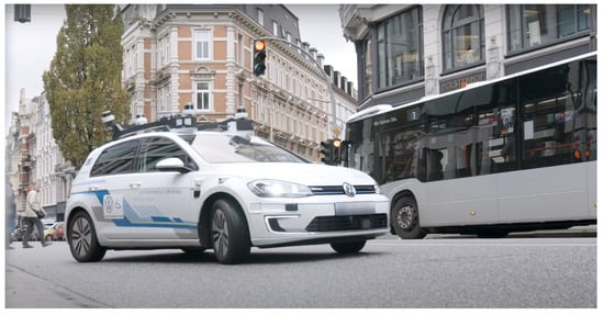
The perception system of the automated vehicle, responsible for detecting and classifying the objects in the scene, has to fulfill the low (0) false negatives requirement, a more difficult one than the low false positives requirement specific to driving assistance systems. The solution for this problem is multiple redundancy, increased accuracy and robustness, along with 360∘ coverage around the vehicle at the sensory and algorithmic levels. To achieve this goal, the UP-Drive vehicle was equipped with the area-view fish-eye camera system (4 RGB cameras) for surround view perception, a front narrow field of view camera for increased depth range and a suite of five 360∘ LiDARs.
2. Proposed Approach for the Enhanced Perception System
2.1. Test Vehicle Sensory Setup
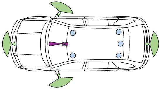
The demonstrator used in the UP-Drive project is based on a fully electric Volkswagen eGolf outfitted with industrial computers in the trunk space, which can take over all controls of the vehicle. The perception task is carried out on a small form factor PC that features a quad-core processor running at 3.60 GHz and a NVIDIA GTX1080 GPU. Figure 2 shows the sensor payload layout used by the enhanced perception solution: area-view system (also known as surround view, increasingly common on new vehicles) comprising of four cameras, one narrow field-of-view (FoV) camera and five LiDAR scanners. Ego-motion data is also available based on vehicle odometry (without GPS).
Figure 2. Sensor payload of test vehicle: 360∘ LiDARs in blue, area-view system with fish-eye RGB cameras in green, narrow FoV camera in purple.
The four area-view (AV) cameras feature 180° horizontal FoV fish-eye lenses, enabling them to capture a surround view of the vehicle. The acquisition of 800 × 1280 px RGB images is externally synchronized between all AV cameras, with very low jitter. The additional narrow FoV camera is mounted in the position of the rear-view mirror and captures 1280 × 1920 px RGB images with a 60° FoV. It is also hardware synchronized with the AV system, complementing detection at longer ranges. Three-dimensional geometric information is captured by the five LiDAR scanners, three of which feature thirty-two vertical scan beams (asymmetrically spaced), while the middle-rear and right-rear scanners use sixteen beams.
Offline calibration
[4][5] of the cameras and LiDARs provides intrinsic parameters of the cameras (radial distortion, focal length) and extrinsic geometric parameters (position and orientation in 3D) of cameras and LiDARs. Camera intrinsic calibrations are done using a standard checkerboard calibration pattern. The extrinsic calibration of the cameras provides the relative positions and orientations of the cameras with respect to a 360° LiDAR master sensor and is achieved with the aid of a set of markers mounted on the walls of a calibration room. The extrinsic 360° LiDAR calibration is also carried out in the calibration room and provides the relative position and orientations of each LiDAR with respect to a chosen master LiDAR (the front left sensor). Finally, the sensor coordinate system is registered with respect to the car coordinate system.
2.2. Perception System Software Architecture
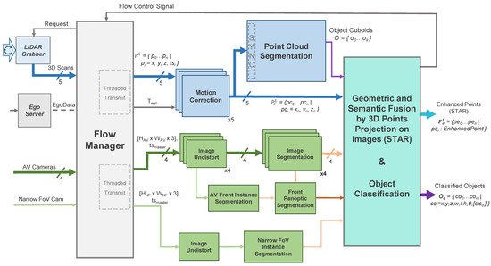
Figure 3 illustrates the enhanced perception system’s architecture, where the necessary operations are subdivided into a series of modular entities, all of which were implemented as plugins in the ADTF Automotive Framework
[6] using the C++ programming language. The data inputs are aggregated by the Flow Manager which controls the two processing chains: the operations on the 3D point cloud (light blue) and those on the 2D images (light green).
Figure 3. Data flow architecture of the proposed enhanced perception system: 3D geometric information (blue, top part) is processed in parallel with 2D camera images (green, bottom part) before the final merger of the two.
The two sensor modalities are handled in parallel on limited hardware by delegating the 3D processing to the CPU and the camera processing to the GPU. The final plugin performs data fusion of the intermediary results, forming the basis for the final detection refinement and classification step. A set of classified objects
Oc, containing both static and dynamic type detections is outputted, along with the semantically enhanced 3D point clouds (STAR)
PLe, each corresponding to a LiDAR scanner
L, which are further used in other modules of the system (e.g., curbstone detection
[7] and localization
[8]). Classified objects
coj are represented as cuboids defined by their center (
x,y,z), dimensions (
w,l,h), orientation (
θ) and ordered classification vector (
[clso]) which features the most likely class predictions. The enhanced points use the
EnhancedPoint data structure (detailed in Algorithm 1), which adds information both from the 2D domain as well as from the 3D segmentation (the object ID and class if the point is part of a segmented detection).
| Algorithm 1: STAR 3D point enhancement representation. |
struct {
float x,y,z;
bool isEnhanced;
uInt8 r,g,b;
uInt16 u,v; \\projection coord.
uInt16 instanceID;
uInt8 semClass;
uInt16 objID;
uInt8 objClass;
} EnhancedPoint; |
2.3. Pre-Processing Functions
The
Flow Manager module performs multiple tasks: data and execution stream synchronization, as well as memory and thread management. Improvements are brought to the system presented in
[9] based on continuous monitoring of the system running in real-time onboard the test vehicle. In order to reduce, as much as possible, the latency between the acquisition of raw measurements and the final results being outputted, we decided to forgo the use of point cloud buffers for each LiDAR scanner as these introduced additional delays due to the behavior of upstream components. Instead, we introduce a data request mechanism to communicate with the raw LiDAR data grabbers. A new data batch is formed by requesting the 360° point clouds from the LiDAR Grabber once processing completes for the current batch (signaled by the Flow Control Signal). The request is based on the batch’s master timestamp, corresponding to the (synchronized) acquisition timestamp of the most recently received set of images,
tsmaster. The response to the Flow Manager’s request consists of point clouds from every LiDAR
L, where the last scanned point
pn in each cloud was measured (roughly) at the master timestamp (consequently, the first scanned point will have been measured approximately 100ms earlier, as the scanners operate at a 10 Hz frequency).
Once all the required inputs are gathered, the Flow Manager plugin bundles the calibration parameters and ego motion data and sends them for processing on two independent execution threads, one for each sensor modality. The ego motion is provided as a 4 × 4 matrix Tego, comprised of rotation and translation components that characterize the vehicle’s movement between the moment of image acquisition going back to the earliest scanned 3D point included in any of the five point clouds. The plugin also performs memory management and handles dropouts in sensor data: the system continues to function as long as the cameras and at least one LiDAR are online, while also being able to recover once offline sensors become available.
Camera images first undergo an
image undistortion pre-processing step that produces undistorted and unwarped images that better represent the scene, based on the camera’s projection model, as detailed in
[3]. While we have experimented with single- and multi-plane representations of the virtual undistorted imager surface, the best results were obtained when considering a cylindrical representation in which the axis is aligned with the ground surface normal. Using look-up tables, this step is performed in 1 ms for each camera.
For 3D data,
motion correction is the process of temporally aligning the sequentially-scanned points
pi to the master timestamp of the data batch (Equation (
1)), thus eliminating the warping induced by ego vehicle movement during the scan (obtaining
pci). Besides correcting geometric distortions, this step also enables a pseudo-synchronization between the two sensing modalities, temporally aligning the point clouds to the moment of image acquisition (represented by the master timestamp)—the unknown movements of dynamic objects in the scene limiting the possibility for full synchronization.
The procedure carried out by the correction plugins (one for each LiDAR
L) is a computationally-optimized version of the one we presented in
[3], completing the task in approximately 2.5 ms, yielding corrected point clouds
PLc: the correction transform
Ci is computed using the matrix exponential/logarithm functions
[10] applied on the ego-motion transform
Tego, based on the time difference
Δi between master and point
tsi timestamps (Equations (
2) and (
3)). To reduce the processing time of each motion correction plugin, we use look-up tables to compute approximations of
Ci, each of which can be applied to small groups of 3D points captured in very rapid succession one after the other, without decreases in quality. We also employ the OpenMP library to perform computations in parallel. This does require a fine tuning of the maximum number of workers allowed to be used by each plugin instance, based on the system load of the host computer. Each worker is assigned a subset of points from the cloud, in order to minimize computational overhead.
2.4. 2D Panoptic Segmentation
We develop a robust, fast and accurate 360
∘ deep-learning-based 2D perception solution by processing images from the five cameras mounted on the UP-Drive vehicle. Our 2D perception module’s goal is to detect static infrastructure such as road, sidewalk, curbs, lane markings, and buildings, but also to detect traffic participants. This is achieved with image segmentation which extracts semantic and instance information from images. We also solve inconsistencies between semantic and instance segmentation and provide a unified output in the form of the panoptic segmentation image. In the case of wide-angle area-view cameras that provide the 360
∘ surround view, a large extent of the scene is captured, but the apparent sizes of objects are smaller compared to narrow FoV cameras. Thus, the detection range of segmentation algorithms of area-view images is limited to the near range around the vehicle. In use cases such as parking or navigation at very low speed, area-view images provide the necessary range. However, detecting distant objects is important when driving at higher speed in urban environment. Therefore, we also utilize the narrow 60
∘ FoV frontal camera, mounted behind the windshield, in order to extend the detection range. A detailed description of our 2D perception solution is presented in
[11].
Our hardware resources are limited and our system requirements impose that our 2D perception solution runs in at least 10 FPS. In order to satisfy these constraints, we develop semantic image segmentation for the area-view images and instance segmentation only for the front area-view image and the front narrow FoV image. Panoptic image segmentation is implemented for the front area-view image. The instance and panoptic segmentation can be easily extended to other views when using more powerful hardware.
For semantic segmentation we implement a lightweight fully convolutional neural network (FCN) based on ERFNet
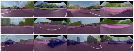
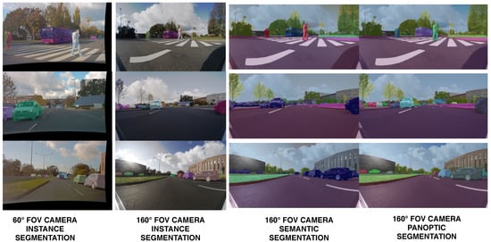
[12], which has an encoder–decoder architecture. Results of the semantic segmentation for the four cameras are illustrated in
Figure 4. For instance segmentation we employ the single-stage RetinaMask
[13] network.
Figure 4. Semantic segmentation of the four area-view images: front, right, rear and left. The semantic perception provides 360∘ coverage, where each image has a 160∘ FoV.
In order to solve conflicts between the semantic class provided by the instance and semantic segmentation, we develop a fusion scheme
[14] for panoptic segmentation. We observe the following problems that are solved by our solution: low-resolution instance masks (
28×28) are upsampled to match the input image resolution and results in raw object borders, semantic segmentation of large objects is problematic and classes belonging to the same category are often confused. The idea is to match pixels from the semantic and instance segmentation at category level and perform a region-growing algorithm in order to propagate the instance identifier and instance segmentation class, which is more stable.
Figure 5 shows the output of the instance segmentation process performed for the two cameras, as well as the panoptic segmentation resulting from the fusion with the semantic segmentation.
Figure 5. Comparison of the front narrow FoV and the front area-view instance segmentation. The apparent sizes of objects is larger in the 60∘ FoV image than the area-view image. By introducing the narrow FoV image, we increase the instance segmentation depth range. We provide instance, semantic and panoptic segmentation on the front area-view image.
2.5. 3D Point Cloud Segmentation
We adopt a two-step strategy for 3D point cloud segmentation: first, the road surface information is extracted from each LiDAR cloud individually, which provides a first separation between LiDAR measurements originating from the road and those from obstacles. This is then followed by a 3D obstacle detection step for which we propose a voxel representation that supports fusion across LiDAR sensors. Thus, we exploit the different viewpoints of each LiDAR scanner in order to obtain a better detection of obstacles in a single pass. Non-road LiDAR points obtained in the first step are fused (and densified) into a single voxel space representation. For each 3D obstacle we provide both the traditional cuboidal representation as well as blobs of connected voxels, which can more accurately capture the occupied space of hanging or non-cuboidal obstacles.
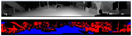
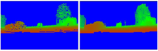
Figure 6 top, illustrates the initial layer/channel representation of LiDAR data on which the road surface detection is carried out, where 3D measurements are ordered by their layer (vertical) and channel (horizontal) angles. Figure 6 bottom, shows the preliminary road/obstacle classification of the panoramic data which takes into account the local slope information.
Figure 6. (Top): Layer/channel representation of the front left LiDAR output (the logarithm value of the inverse depth is shown for visualization), (Bottom): Preliminary classification results (road—blue/obstacles—red).
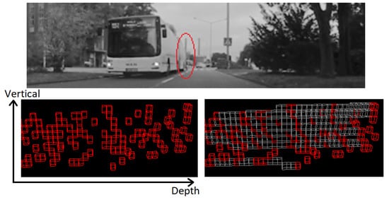
The voxel representation covers a space of interest centered on the ego vehicle, with a square shape in the bird’s-eye view. The top view area covered is 160 × 160 m, with a voxel size of 16 × 16 × 16 cm, with the ego vehicle in the center. Each obstacle measurement is inserted into the voxel space, and voxels are marked as obstacles accordingly. However, one important issue must be accounted for: depending on the orientation of an obstacle facet relative to the LiDAR, or the distance from the ego car, obstacle measurements that are adjacent in the layer/channel space might not be connected in the Euclidean voxel space (Figure 7).
Figure 7. The farthest part (encircled with red, (top image)) of the lateral side of the bus has consecutive LiDAR measurements that are not connected in the voxel space ((bottom-left image): side view, red voxels). After densification, the introduction of the intermediate voxels (gray) provides an increased level of connectivity ((bottom-right image): side view).
The densification of the voxel space is achieved by inserting intermediate obstacle voxels between the originally-adjacent LiDAR measurements. Both vertical and horizontal connectivity are exploited. Two obstacle measurements are adjacent in the following configuration:
- (a)
-
(vertical) Adjacent layers and the same channel, and the 3D distance between the measurements is below a threshold
- (b)
-
(horizontal) The same layer and adjacent channel values, and the 3D distance between the measurements is below a threshold.
For the second situation (horizontal connectivity), an additional constraint must be imposed regarding the planarity of the surface where the intermediate voxels are inserted. This is needed in order to avoid unwanted joining of nearby independent obstacles. The local angle of the 3D measurements is evaluated along each layer (from the previous, current and next channel measurements). Intermediate voxels are inserted only for those obstacle measurements where this angle is close to 180 degrees (should belong to a surface that is close to planar). Computing the location of intermediate voxels that must be inserted can be quickly solved using Bresenham’s line algorithm (3D version).
By densifying the voxel space, we ensure that measurements adjacent in the panoramic representation are connected, by having intermediate voxels forming uninterrupted paths between them even in cases with no intermediate measurements. The intermediate and occupied voxels allow the extraction of 3D obstacles as connected components. These are found through a breadth-first search which generates a set of candidates for which multiple features (size, voxel count, LiDAR 3D point count, etc.) are calculated, which allows for some of them to be discarded if their features are outside of expected ranges. Finally, for each obstacle blob, the oriented cuboid is computed with a low complexity approach based on random sample consensus fitting of L-shapes, described in
[15]. Results are shown in
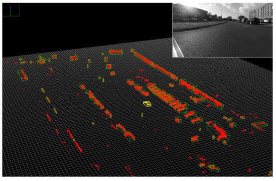
Figure 8.
Figure 8. Individual obstacles are detected in the voxel space (red voxels), and valid obstacles are represented as oriented cuboids (green).
2.6. Low-Level Fusion: Spatio-Temporal and Appearance Based Representation
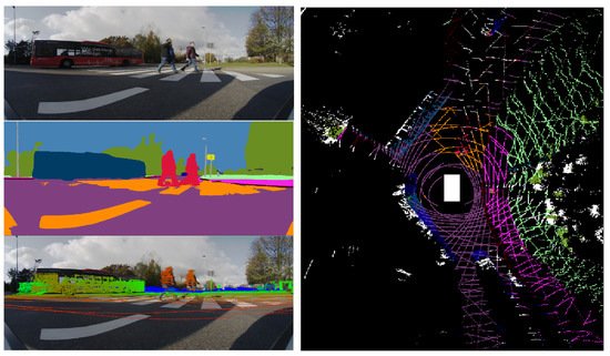
The Geometric and Semantic Fusion module aggregates data from the two execution threads and generates the spatio-temporal and appearance-based representation (STAR) by projecting all the motion-corrected 3D points onto every raw and segmented image using the associated calibration parameters of each sensor (see Figure 9). This process, which attaches RGB and semantic information to all points that project onto the 2D data, can become a computational bottleneck, prompting us to use a complex, multi-threaded execution scheme, that takes place for each received 3D cloud once 2D segmentation results become available.
Figure 9. The Low-level fusion process: Raw and semantic information from the camera is fused with the projected 3D points (left column, from (top) to (bottom)) to produce an enhanced 3D point cloud (STAR, (right)).
Equations (
5)–(
7) present the mechanism for projecting 3D points
pci onto the unwarped images based on the cylindrical image plane representation, using the camera intrinsic matrix
Kcam and the 3D coordinate transform
TLcam, provided by the calibration procedure for each pair of camera
cam and LiDAR
L. Here, the function
point_to_cylinder computes coordinates at which rays extending towards
pci intersect the cylindrical surface of the (modelled) image plane.
Occlusion handling is an important practical problem which arises during sensor fusion and we address it with two different approaches. They both use semantic and depth information: one fast approach relying on projecting onto a low-resolution virtual image and one more costly approach which applies corrections to each image column.
Semantic labels from occluding objects seen in camera images can be mistakenly propagated to 3D points belonging to the occluded objects during the information fusion process between the LiDAR point cloud and semantic segmentation images. The occlusion handling algorithm presumes objects to be either static or that their position has been corrected (which in turn requires additional information).
The
sparse depth map (raw) representation, denoted by
D(x;y) is obtained by projecting the 3D measurements onto each image, sparsely adding distance information to pixels where possible, with the other pixels marked accordingly. An intermediary operation aims to increase the density of the depth map by considering cells of fixed size
s (e.g., 10 × 10 px) and constructing a lower-resolution depth map by taking the minimum distance in each cell. In practice, this can be implemented by creating the low-resolution image directly, which reduces computation time significantly and achieves the same results. The low-resolution image has values equal to the local minimum in an
s by
s box:
Besides sparsity, another common problem is the lack of measurements due to non-reflective surfaces of objects from the scene. To address this issue we propose two correction schemes: one based on the dilation of the measurements and the other based on convex hull estimation.
Since LiDAR point layers fall farther apart onto objects which are closer, measurements are dilated in the horizontal and vertical direction based on the distance. The dimensions of the dilation kernel are given by: drows=min(4;20/dist),dcols=min(1;5/dist), where dist is the distance of the 3D point, making the the window size inversely proportional to it (the scalar values were selected empirically, with a higher kernel size needed on the vertical direction due to higher sparsity). This operation does not affect the execution time significantly since it only applies to points within a 20 m range.
Semantic information allows us to treat each object class differently. Occluding objects can only be from the following semantic classes: construction, pole, traffic light, traffic sign, person, rider, car, truck, bus, train, motorcycle, bicycle, building or vegetation. Point measurements from other classes, such as road or lane markings, cannot occlude other objects.
Occlusions are detected using the generated dense depth map by simply marking projected points which have a larger distance than the corresponding cell from the depth map as occluded. Semantic classes associated to such points should be ignored as they originate from an occluding object. Figure 10 illustrates the resulting low-resolution depth map.
Figure 10. Low resolution depth map and its corrected version - scene depicts a car close by on the left, a car in the middle farther away and foliage on the right. Color encodes the distance from red (close) to blue (far), up to 20 m. Positions with no measurements default to infinity.
An alternative, more computationally costly, approach was also implemented. It performs a column-wise completion and relies on estimating the lower envelope of the measurements for a single object based on the semantic labels. More precisely, we consider each column from the depth map and segment it according to the semantic labels. For each segment, after finding the lower envelope we update the depth values to match those from the envelope. This predicts the depth linearly between two measurement points and eliminates farther measurements.
2.7. STAR-Based Classification and Enhanced Detection
Once the LiDAR measurements are enhanced with semantic information while also considering occlusions, the process of object classification can be performed in order to provide class labels to each object cuboid. In order to increase robustness to outliers caused by mislabeled 3D measurements (such as those on the border of dynamic obstacles or on thin objects), a statistical method is adopted. The following steps are performed for computing the semantic class for each detected object:
-
The semantic class is first transferred from the individual 3D measurements to their corresponding voxels, handling conflicting measurements by labeling the entire containing voxel as unknown
-
A semantic class frequency histogram is generated for each 3D obstacle, based on the contained voxels, enabling a statistical based approach for the final decision step:
- -
-
The most frequent class is selected as the 3D object class
- -
-
Up to 3 additional, most likely classes can be also provided, allowing further refinement of the object class during subsequent tracking processes
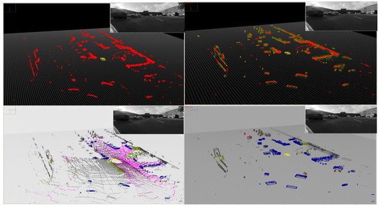
Results for obstacle classification are presented in Figure 11. The enhanced semantic information of the 3D points can be further exploited to refine the detected objects by separating grouped obstacles of different classes or different instances of the same class. A strategy was developed to analyze the distribution of classes or instances in an obstacle. If at least two dominant classes/instances are detected (frequency over a threshold), then new centroids of individual obstacles are computed and voxels are reassigned to each obstacle (nearest centroid).
Figure 11. Results of Object Detection and Classification. Top-Left: Input LiDAR Point Cloud, Bottom-Left: STAR Point Cloud, Top-Right: Segmented Objects, Bottom-Right: Classified Objects.