Distributed Deep Learning: From Single-Node to Multi-Node Architecture

Distributed Deep Learning: From Single-Node to Multi-Node Architecture: History

Please note this is an old version of this entry, which may differ significantly from the current revision.

Contributor:

During the last years, deep learning (DL) models have been used in several applications with large datasets and complex models. These applications require methods to train models faster, such as distributed deep learning (DDL). Local parallelism is considered quite important in the design of a time-performing multi-node architecture because DDL depends on the time required by all the nodes.

deep learning
frameworks
CPU
GPU
distributed computing

1. Introduction

The explosion of data, in terms of computation capabilities, offers new options to analyze data through more complex models. Such models are Artificial Neural Networks (ANN) that are composed of several layers. These models represent the main component of the DL domain, which is a growing trend for both scientific research and enterprises that want to understand their data or automate tasks such as face recognition.

In DL, some particular tasks focus upon complex data, such as images and videos. Image and video classification are Machine Learning (ML) tasks that are carried out by models trained with data in order to recognize predefined identities in images such as animals or handwriting. DL performs well on these kinds of tasks. These DL tasks use a particular kind of layer, named Convolution, in their architecture. Convolution processes a 3D structure—an image that has red, green, and blue channels, identified by their row and column indices, on each of its pixels—in order to extract features such as edges in images. These features are used as inputs to classical Neural Networks.

To train a model for classification, two steps are required: (1) the learning, which involves training the model to fit the data, and (2) the validation, which involves evaluating the the model (e.g., accuracy). The training uses the forward propagation which works by successively applying each layer to an input in order to make a prediction regarding that input, and the back-propagation which consists of measuring the prediction error in order to update the model from the last layer to the first. The model can therefore be used to make predictions or to be tested, which uses only the forward propagation.

The increase in data also occurs in image and video classification tasks requiring the alternative processing of a significant amount of data. Such an alternative is called Distributed Computing, a well-known and developed field. Even if the scientific literature could successfully apply Distributed Computing in DL, no formal rules to efficiently process data in terms of time exist. Therefore, the focus of the current work is how to efficiently distribute a DL task without having access to a dense GPU cluster because of the cost.

As a first step, this analyzes how to efficiently distribute a DL task in order to decrease the processing time. Multi-threading techniques have been well-optimized in libraries such as cuDNN and MKL-DNN, which are used by frameworks such as TensorFlow and PyTorch. Moreover, multi-processing techniques have been implemented in libraries such as Horovod ^[1]. Taking into account local parallelism can speed up the DDL, does not require intense network communication, and outperforms Horovod. To this end, sequential processing was measured to serve as a baseline. Then the processing was parallelized on a single machine with different setups to choose the highest acceleration measured by a speedup metric. The best setup (i.e., less computing time) is used as a local strategy (i.e., on a single machine) in order to distribute the load across machines, resulting in an efficient DDL.

2. Development

Our experimental setup is based on a benchmark ^[2] of DL frameworks as a baseline for speeding up calculation. The benchmark recommends using the pyTorch framework and focuses on two use cases that this work therefore also uses. This section is dedicated to explain and detail the DL task and the different setups used. In this entry, the acceleration factor called speedup is used and defined as $\frac{{\bar{t}}_{b}}{\bar{t_{s}}}$ , where ${\bar{t}}_{s}$ and ${\bar{t}}_{b}$ , respectively, stand for the average time of the setup and the baseline. The baseline depends on the device (CPU or GPU). It corresponds to the time needed to process the DL task sequentially on a single CPU core or GPU.

Table 1 reports the baseline times depending of the device and the use case. For example, a parallelism setup which is two times faster than the baseline provides a speedup value of 2.

Table 1 : Baseline times (seconds).

Process Mode	ComplexSmall	SimpleBig
Sequential single-core CPU	629.73	879.38
Sequential single GPU	34.25	121.82

2.1. Use Cases

The two use cases are:

ComplexSmall uses the VGG16 ^[3] CNN architecture on the small dataset;
SimpleBig uses the AlexNet ^[4] CNN architecture on the large dataset.

The architectures have been adapted to support a three-class problem.

2.2. Training Task

The training task for the image classification problem has to address how to feed the neural network with images. The latter have to be pre-processed in order to fit the input required by neural networks (AlexNet and VGG16 require an input of 224×224). In this work, such pre-processing is designed based on the original publication of the selected CNN instead of designing the most accurate model. This is why input images are pre-processed to 224×224 with the 3 RGB channels. The goal is to measure and quantify the resource usage of a common learning task. The image pre-processing pipeline follows the sequence:

Image crop/scaling to 224×224;
Random horizontal flip transformation;
RGB-normalization with μ=(0.485, 0.456, 0.406), σ=(0.229, 0.224, 0.225);
Conversion to a tensor data structure.

The optimizer is the mini-batch gradient descent with a learning rate α=0.001 and a momentum μ=0.9. The loss is computed with the cross-entropy method.

2.3. Setups

In this section, parallelism strategies are examined to determine when they can be applied and what the conditions are.
In addition, the communication mechanisms on the network are discussed in order to design DDL.

2.4. Parallelism

Parallelism consists of the simultaneous execution of multiple computations. There are two main mechanisms in the CPU:

Multi-threading: a single application that runs only once as a process---a program loaded in memory---but that simultaneously executes blocks of instructions, with each block being a thread. The process memory is shared among all threads;
Multi-processing: the same application runs multiple times (on GNU/Linux systems, this application duplicates its whole execution context)
and the operating system simultaneously executes each instance of the application, which is called concurrency. Each instance can be multithreaded.

Multiple simultaneous executions are carried out in data parallelism. The model is replicated into each execution, therefore increasing the amount of memory used. Each execution then loads the data and feeds its own Deep Learning tasks. After this step, synchronization of the gradient occurs and concurrency stops in order to ensure that all models---each execution---are identical in memory.

The model is split among available devices in model parallelism. This technique is required when the whole model cannot be loaded in memory on a single device. For example, a neural network is split on a computer composed of two GPUs.
At time t=0, the process loads a batch of data from the storage device.
At time t=1, the first GPU receives and feeds the first part of the neural network with the data while the process loads a second batch of data.
At time t=2, the second GPU receives and feeds the second part of the neural network with the output of the first GPU (i.e., the result of the first batch of data), the first GPU feeds the first part of the model with the second batch, and the process load a third batch of data.
At the time t=3, the output of the second GPU produces the final output and the gradient can be computed.
Then the model is updated with the back-propagation algorithm.
Finally, the training repeats the sequence and continues to load data and feeds the neural network.
Pure model parallelism is less efficient than loading the model upon a single device because of the transfer overhead. Pipelining ^[5] the batch, however, makes the overhead less costly than the gain of parallelism, depending on the batch size and the model complexity. Pipelining on the batch consists of dividing the batch into distinct sub-batches. Each sub-batch passes through each device, and therefore into each part of the model. While the first sub-batch gets processed by the second device---it has already been processed by the first device---the second sub-batch is being processed by the first device.

In the setups, model parallelism on GPU makes sense: while the CPU prepares data, the first GPU takes approximately the same time as the second GPU to process the respective data due to the split of matrix operations, GPUs having the same capabilities. This of course depends on the balance of the neural network distribution between the GPUs. Neural network architectures (AlexNet and VGG16) are divided into two equal parts (number of layers and synchronous operations such as pooling). AlexNet is split after the 4th convolution layer while VGG16 is split after the 8th convolution layer. On a CPU, such an approach would only result in overhead because it has to transfer data without any gain in processing data on another similar CPU. The CPU remains slow on matrix operations.

Because of the environment---the available hardware---multi-process data parallelism on a GPU is a bad idea. Multiple processes attempting to access the same GPU are actually discouraged by the hardware designer and usually results in memory overflow. The GPU API requires state information called a context. A context is linked to the data stored in the GPU and the process that uses the data. Multi-process can lead to a situation where the sum of the data linked to contexts overfit the GPU memory. To bypass this limitation, the designer proposes their multi-process service which acts as an interface between the GPU and the processes. Nevertheless, an official example of code (the file simpleIPC_mod.cu of CUDA) contains a comment about using multi-process: "Multiple processes per single device are possible but not recommended."
This limitation only enables one process to be carried out per GPU. Data preparation on the CPU must be fast in order to quickly feed the GPU and to overcome this limitation of the process. In this setup, the difference between data and model parallelism resides in synchronization. In the data parallelism setup, after each result is received from the device, processes have to synchronize, in contrast with model parallelism which does not require synchronization, due to its sequential flow. Model parallelism efficiency depends on the transfer time and the waiting time between the synchronization mechanism of GPUs---i.e., when the GPU i+1 has finished processing and waits for the result to be delivered from the GPU i.

The multithreaded data parallelism on a CPU is applied in a single process. Data parallelism is induced by splitting a batch of size n into k smaller batches of size n/k, each trained into k distinct threads. Each thread works on a replica of the CNN architecture.

2.5. Network Protocol Family

Instead of using a whole framework, including both a programming model and load distribution, a simple network protocol can be used to distribute a computation load. The advantage of using such a protocol is that it reduces the size of the software stack used and simplifies the execution, but this also increases the lines of code required for computation because of the need to use proper network functions. Four protocols are considered:

Socket: Using TCP/IP or UDP communication only. With UDP, network packets are smaller but if the network is fully used, data will be dropped, unlike in TCP/IP, which automatically adapts its behavior. In this kind of implementation, the developer has to design how and which information to send to other nodes;
Remote Procedure Call (RPC): A protocol designed to call a remote procedure or function with parameters. This protocol enables the abstraction of an underlying connection such as TCP/IP and easily allows executing a remote function;
Remote Direct Memory Access (RDMA): Enabling direct access to the memory of a remote computer without involving the operating system. It is characterized by a high throughput with low-latency networking. A disadvantage is that RDMA does not notify the remote computer that a request has been conducted. It is a single-sided method of communicating;
Message Passing Interface (MPI): Not only a protocol but also a norm that specifies how to send messages between remote computers. Like RPC, MPI offers an abstract layer to the developer, but is also able to efficiently send messages among a cluster of computers with different underlying technologies (e.g., RDMA, TCP/IP, ...).

An alternative is to implement the software inside a map-reduce framework. This is a parallelism design pattern enabling the manipulation of a large amount of data by spreading the data and the processing among a cluster. This pattern is well known and used by large companies such as Amazon and Facebook. Spark is a technology from 2014 built upon Hadoop and aimed at speeding up data processing. It runs the whole execution in RAM in real time, unlike Hadoop. It only uses persistent storage when the RAM is not sufficient.

2.6. Proposed Approach

This work assumes that a fast distributed process can be achieved if all computers involved in the DDL perform locally. That is to say that each computer executes the DL task with the parallelism paradigm that is faster on it. To identify the fastest parallelism and the configuration (e.g., number of threads), the speedup metric is used. Figure 1 is a diagram of two computers---the workers---that apply model parallelism, each on two GPUs. Between the nodes, data parallelism is used with the local replication of the datasets. After the processing by the GPU of a batch of data, the average gradient is synchronized through MPI messages. The transfer of data between GPUs on a same host does not require to go through the CPU if GPUs are interconnected. The pyTorch framework supports this feature.}

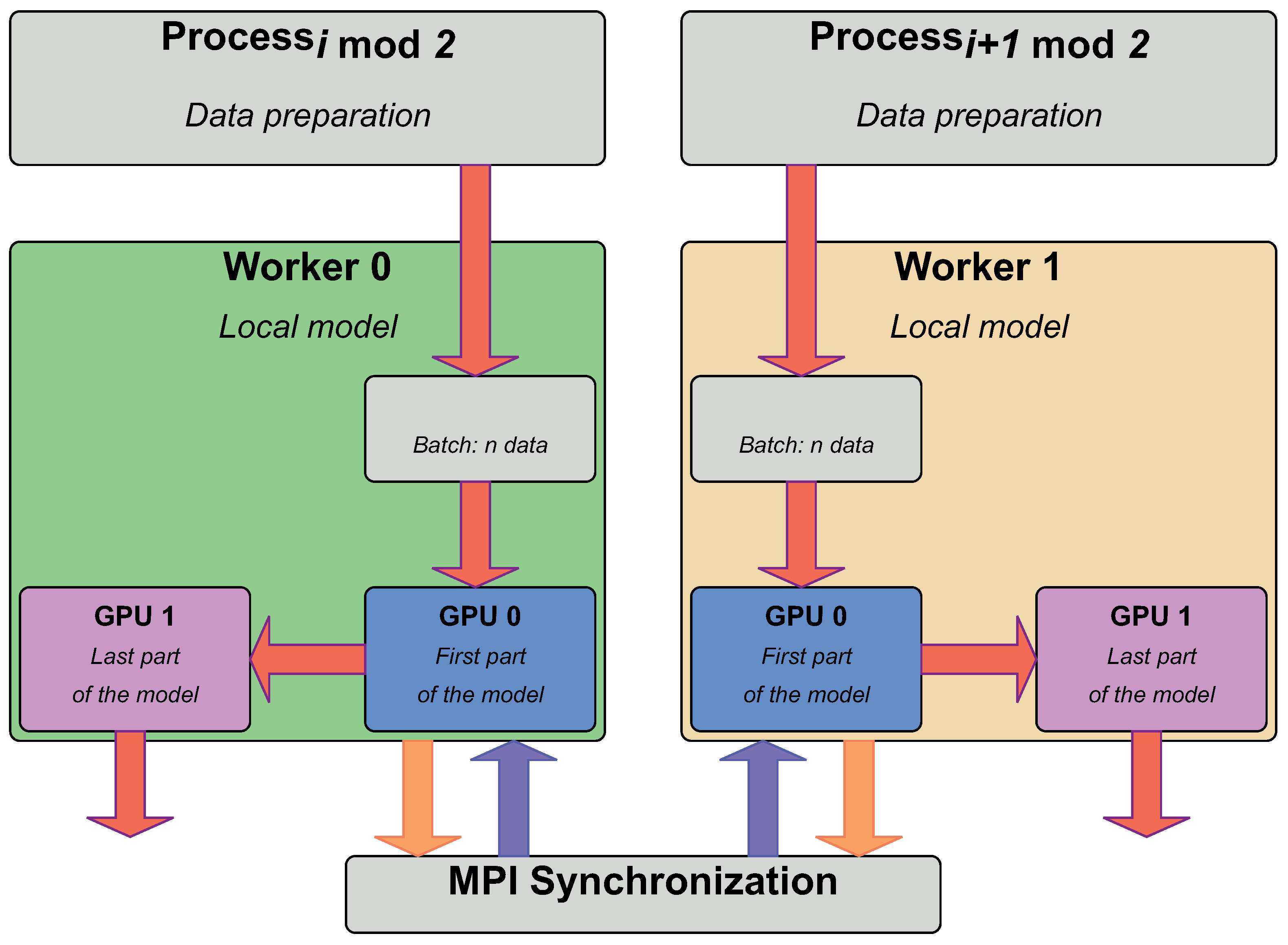Figure 1. Diagram of DDL via MPI with local (green and orange areas) model parallelism. The worker 0 (resp. 1) has even (resp. odd) processes that load an independent non-overlapping batch of data from the same training set. Then model parallelism applies and produces the output. Instead of directly updating the model with the gradient, it is averaged locally and sent to the other worker. Then the gradient is averaged and the local model of each node is updated at the same time. That is, the two parts of the model that are stored on the two GPUs are updated.

The CPU and the RAM utilization rates are measured by the pidstat utility. They are respectively the total percentage of CPU time used by the task and the tasks currently used share of available physical memory. The other measurements are made with the sar utility.

3. Findings

DDL is a tool to speed up the execution of a DL task. In the scientific literature ^[6], works distribute the workload on machines mainly using MPI or Apache Spark. The problem of DDL is the cost of network communication because the more the task is distributed to compute nodes, the more the network load increases. In this entry, the distribution of DL tasks is performed with MPI which has been shown to perform better ^[2] than tools based on the MapReduce paradigm (e.g., Apache Spark). Usually, MPI is used to distribute the computing load over the entire infrastructure. Therefore, there are several computing processes on the same machine. This is not the case in this work, MPI runs only one computing task on a single machine. The computing task will itself create several processes/threads in order to allow them to exchange information directly. For example, on the GPU, the data will be associated with a single execution context. This avoids loading and unloading data unnecessarily.

The DDL method used is based on the assumption that a fast local (on each machine) parallelization allows to speed up the whole distributed task. This is why it is important to understand: how best to parallelize locally. To this end, data parallelism, model parallelism, and a hybrid approach have been considered. Parallelism was applied on the CPU and the GPU with two use cases to highlight the effect of a complex model and the effect of the amount of data. The results have shown that DDL can be slower than pure parallelism on small datasets. On a single computer, the multi-process data parallelism is faster on the CPU and the model parallelism is faster on the GPU.

There are studies that have already focused on how to decompose a DL task in a distributed way by exploiting different parallelization methods including a hybrid approach ^[7]. The problem is that by doing this, the network communication is intensified. For example when the neural network is divided ^[8] on several machines. Each machine has to communicate both to exchange the gradient but also to exchange data between the different parts of the model. However, network communication is the major problem of DDL. Several methods ^[9]^[10]^[11]^[12]^[13]^[14]^[15] can be used to reduce the amount of network traffic, but this comes at a cost in terms of accuracy.

The proposed approach takes advantage of parallelization and distributes the load using MPI. The results of this DDL methodology show not only that the computation has been accelerated but also that the required network communication is low, in contrast to the state-of-the-art framework called Horovod ^[1]. In addition, Horovod is outperforming in terms of acceleration. Future work focuses on a larger scale distribution and the effect that data location has on DDL speedup.

4. Conclusions

A novel way to speed up the Distributed Deep Learning has been proposed by focusing on how parallelism is implemented on computers. This customized approach speeds up calculations, saves time and reduces network communication. Future works are to exploit the approach of this entry on a cloud and an edge computing infrastructure, as well as to propose a deployment method for Distributed Deep Learning. It is also interesting to understand how the location of the data affects the results.

This entry is adapted from the peer-reviewed paper 10.3390/electronics11101525

References

Sergeev, A.; Del Balso, M. Horovod: Fast and easy distributed deep learning in TensorFlow. arXiv 2018, arXiv:1802.05799.
Ben-Nun, T.; Hoefler, T. Demystifying Parallel and Distributed Deep Learning: An In-Depth Concurrency Analysis. ACM Comput. Surv. (CSUR) 2019, 52, 1–43.
Lerat, J.S.; Mahmoudi, S.A.; Mahmoudi, S. Single node deep learning frameworks: Comparative study and CPU/GPU performance analysis. In Concurrency and Computation: Practice and Experience; John Wiley and Sons Ltd.: Chichester, UK, 2021; p. e6730.
Teerapittayanon, S.; McDanel, B.; Kung, H.T. Distributed deep neural networks over the cloud, the edge and end devices. In Proceedings of the 2017 IEEE 37th International Conference on Distributed Computing Systems (ICDCS), Atlanta, GA, USA, 5–8 June 2017; pp. 328–339.
Disabato, S.; Roveri, M.; Alippi, C. Distributed Deep Convolutional Neural Networks for the Internet-Of-Things In IEEE Transactions on Computers; IEEE Computer Society: Washington, DC, USA, 2021; Volume 70, pp. 1239–1252.
Cong, G.; Bhardwaj, O. A hierarchical, bulk-synchronous stochastic gradient descent algorithm for deep-learning applications on GPU clusters. In Proceedings of the 2017 16th IEEE International Conference on Machine Learning and Applications (ICMLA), Cancun, Mexico, 18–21 December 2017; pp. 818–821.
Hashemi, S.H.; Jyothi, S.A.; Campbell, R.H. TicTac: Accelerating Distributed Deep Learning with Communication Scheduling. arXiv 2018, arXiv:1803.03288.
Tsai, C.Y.; Lin, C.C.; Liu, P.; Wu, J.J. Communication scheduling optimization for distributed deep learning systems. In Proceedings of the 2018 IEEE 24th International Conference on Parallel and Distributed Systems (ICPADS), Singapore, 11–13 December 2018; pp. 739–746.
Wen, W.; Xu, C.; Yan, F.; Wu, C.; Wang, Y.; Chen, Y.; Li, H. Terngrad: Ternary Gradients to Reduce Communication in Distributed Deep Learning. Adv. Neural Inf. Process. Syst. 2017, 30, 1509–1519.
Sattler, F.; Wiedemann, S.; Müller, K.R.; Samek, W. Sparse binary compression: Towards distributed deep learning with minimal communication. In Proceedings of the 2019 International Joint Conference on Neural Networks (IJCNN), Budapest, Hungary, 14–19 July 2019; pp. 1–8.
Kuang, D.; Chen, M.; Xiao, D.; Wu, W. Entropy-based gradient compression for distributed deep learning. In Proceedings of the 2019 IEEE 21st International Conference on High Performance Computing and Communications, Hyderabad, India, 17–20 November 2019; pp. 231–238.
Li, S.; Hoefler, T. Near-Optimal Sparse Allreduce for Distributed Deep Learning. arXiv 2022, arXiv:2201.07598.

© Text is available under the terms and conditions of the Creative Commons Attribution (CC BY) license; additional terms may apply. By using this site, you agree to the Terms and Conditions and Privacy Policy.