A water supply system is considered an essential service to the population as it is about providing an essential good for life. This system typically consists of several sensors, transducers, pumps, etc., and some of these elements have high costs and/or complex installation. The indirect measurement of a quantity can be used to obtain a desired variable, dispensing with the use of a specific sensor in the plant. Among the contributions of this technique is the design of the pressure controller using the adaptive control, as well as the use of an artificial neural network for the construction of nonlinear models using inherent system parameters such as pressure, engine rotation frequency and control valve angle, with the purpose of estimating the flow.
1. Introduction
Water is a natural resource of fundamental importance for the survival of humans and other living beings, and a good as relevant as this must be preserved in relation to its conscious use. The problem of water waste, not only in domestic waste (excessive use of water to wash sidewalks, time-consuming cleanliness with open registers, etc.) but mainly in waste from the point of view of supply systems (leakage in pipes, for example) makes the obstacle much higher. The feasibility of means that mitigate waste through an efficient distribution to a given location is extremely important. Thus, in the context of water distribution to the population, there is a need for an efficient resource distribution system capable of meeting urban and rural demands. In this way, a water supply system is defined as the set of works, equipment and services intended to supply drinking water to a community for the purposes of domestic consumption, public services, industrial consumption and other utilities [
1]. This water supplied by the system must be in sufficient quantity and of the best quality from a physical, chemical and bacteriological point of view.
A water supply system (WSS) represents the entire process of supplying treated water, ranging from obtaining it to its use by the population. For this, a WSS uses a set of equipment, works and services, whose objective is to supply the water demand of a given population. Thus, the typical elements of a WSS are catchment (from a spring), pumping station, pipeline, water treatment station (WTS), reservoirs, distribution network and finally household connections (consumers).
The water stored in the distribution reservoir after the intake, elevation/adduction and WTS steps can be pressurized in the pipeline in two ways: by gravity and/or by a motor-pump set. By gravity, water is transported to the consumer without the need to use electricity. On the other hand, in the second case, an artificial impulsion system is needed, that is, by a hydraulic motor-pump coupled to an electric motor and/or by means of a booster (BST) [
1].
In many practical cases, the non-linearity of the topography of a region causes the water pumping systems to operate in such a way as to meet these unevennesses, as in cases where there are low areas (topographic regions with low topographic elevation) and high areas (topographic regions with high topographic elevation in relation to low areas). In the case of the high zone, the pumping station, located in the low zone, must increase the pumping head to supply the high zone region. However, this increase causes an excess of pressure in the low zone and, therefore, tends to increase leakage losses and maintenance costs due to pipe rupture [
1,
2].
To solve excess pressure in the low zone and avoid damage to pipes and other installations, there are some solutions to be adopted: one of them is the installation of control valves (pressure-reducing valves or PRVs), automatic or not, with the purpose of modifying the pressures at certain points in the network. This solution is usually adopted, as pumps operating in water supply systems generally work at their nominal speed.
Another alternative is the application of mechanisms to control the rotation speed of electric motors and consequently the hydraulic energy supplied by the pumps. For this purpose, frequency inverters are generally adopted [
2,
3]. These devices convert a voltage into another with desired (controlled) amplitude and frequency. When used to drive a motor-pump set, the frequency inverter can manage the electrical and hydraulic parameters of a pumping station, because by regulating the rotation speed, it also regulates the head (pressure), flow and associated electrical power [
4]. The energy released to promote the increase in flow and hydraulic pressure depends on the rotation speed of the pump set.
Several techniques can be used to promote the control of the frequency inverter applied to WSS for pressure management to keep it stable and contribute to the reduction in losses (electrical and hydraulic). The benefits of pressure control are to increase the useful life of pipes and accessories, increase system reliability, reduce hydraulic transients and reduce wasted electrical energy [
1]. For a supply system to have a satisfactory technical and economic performance, it is necessary to perform pressure control. The uniformity of pressure in the distribution network, through this control, reduces the frequency of ruptures, excessive water consumption induced by pressure and the volume lost in leaks.
Several technologies can be used to measure the main physical quantities in WSS. The flow rate, which is of greater interest in this work, can be measured using technologies such as electromagnetic and ultrasonic, among others [
5,
6]. Other techniques can also be used to measure the flow, such as the equations that characterize the operation of a pump (pressure–flow curve). However, the use of this estimation method requires constant system calibrations, since they are based on the constructive characteristics of the pump, which wears out during operation, varying its characteristics over time [
7].
2. Artificial Neural Networks in Water Supply Systems Development
2.1. Soft Sensor
In recent decades, soft sensors have established themselves as a valuable alternative to traditional means for the acquisition of critical process variables, system monitoring and other tasks that are related to industrial process control [
8]. These virtual sensors generally help regarding the unavailability of (real) hardware sensors in various industrial segments, thus allowing for less occurrence of failures and better control performance. Soft sensors are emerging as a viable alternative for the real-time monitoring of parameters that either lack a reliable measuring principle or are measured using expensive online sensors [
12]. The purpose of a soft sensor is to estimate a variable that is not directly measured but that is related by a suitable model to several other process variables that are directly measured. Thus, for the context of applicability in WSS, the basis for the development of the soft sensor used is the ANNs (artificial neural networks). The option for the developed technique was based on some properties of the ANNs in which they were decisive for the adoption of this technique, such as: (a) no need for mathematical models; (b) generalizability; (c) pattern classification; and (d) learning, among others [
7].
2.2. Indirect Measurements
Several technologies can be used to measure the main physical quantities in WSS. The flow rate, which is of greater interest in this work, can be measured using technologies such as electromagnetic and ultrasonic signals, among others. Regarding technologies that employ electromagnetic principles, associated equipment has higher acquisition and installation costs, depending on the installation diameter and, consequently, on the volume to be measured [
5,
6].
Other techniques can also be used to measure the flow, such as the equations that characterize the operation of a pump (pressure–flow curve). However, the use of this estimation method requires constant system calibrations, since they are based on the constructive characteristics of the pump, which wears out during operation, varying its characteristics over time [
7]. Given the various studies presented, it is important to use techniques that eliminate (or mitigate) the situations, and indirect measurement techniques can be very useful in this regard.
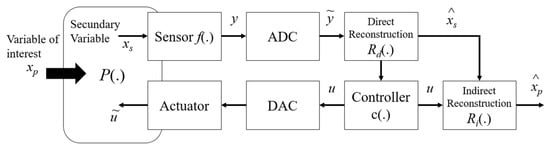
In general, indirect measurements estimate the main variable (or quantity or magnitude) of an electrical signal obtained by directly measuring a secondary variable that is related to the main variable. The realization of an indirect measurement assumes a mathematical model that describes the association between the quantities involved and generally, the relationship between the secondary variable and the main variable is described by differential equations.
Figure 1 illustrates a detailed flowchart of a feedback measurement system adapted from the model proposed by [
16], in which the measurement means
P(.) is dynamically related to the primary variable,
xp, the secondary variable,
xs and the actuation signal,
u.
Figure 1. Generic diagram of a measurement feedback system adapted from [
16].
3.3. Adaptive Control
In today’s language, the term adapt means to modify behavior according to new circumstances or situations. In the engineering context, adaptive control can be defined as a control technique that could change its behavior according to changes in parameters, in the dynamics of a process or by disturbances that affect this system [
15]. Thus, a fixed gain controller (PID for example) is not an adaptive system. An adaptive controller must have the ability to update its control law by changing its gains (or parameters) in real time. In applications involving WSS, external parameters such as temperature, equipment wear and disturbances can alter the system’s operational dynamics. Thus, the use of controllers with static gains, in these scenarios, ends up not being convenient because they are tuned considering that the system is invariant in time and/or only for a specific operating range. Furthermore, the existence of noise and interference from different sources can directly influence the controller’s performance and, in the worst cases, lead to instability in the system [
4]. To control these categories of system, controllers with adaptive gains stand out from those with static gains, as they could modify their parameters according to the changes suffered by the system [
7,
14].
Direct Adaptive Control
Adaptive controllers can be divided into two large groups: direct and indirect. In the direct method, the controller gains are estimated directly from a pre-established reference model; that is, it is not necessary to carry out the identification of plant parameters [
4]. Considering a reference signal
r and an output
y, in the direct method, the controller gains (vector
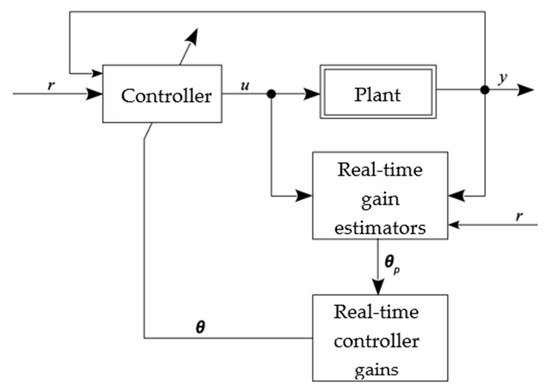
θ) are estimated directly, usually from a pre-established reference model; that is, there is no need for direct estimation of the plant parameters. In the indirect method, the plant model is determined as a function of the unknown plant parameter vector, requiring a real-time estimator, using the input and output of plant signals. Therefore, the generated model is treated as true, and its parameters are used for the calculation of controller variables.
Figure 2 illustrates the representation of a direct adaptive controller.
Figure 2. Direct adaptive controller.
For the direct adaptive control method, most works use the Adaptive reference model controller (MRAC). In this controller, the plant output signal is compared with a model output reference signal, generating a tracking error (ε). Using a cost function, the controller parameters are adjusted based on this error, causing the plant output signal to converge with that of the reference model. The matching condition is reached when ε is equal to zero. The controller parameters are adjusted based on this error, converging the plant output signal to that of the reference model. Generally, for this cost function, the MSE (mean squared error) is the standard adopted [
4].
This entry is adapted from the peer-reviewed paper 10.3390/s22083084