The number (and quality) of sensors used to collect data in different contexts have been steadily growing. Even complex environments, such as agricultural areas, are now being “sensed” via a wide variety of equipment, generating vast amounts of data that can be explored to provide useful information about the area being observed. As a result, the number of studies attempting to explore the wealth of information contained in the sensed data have increased^[1][2][3]. However, it is often challenging to translate the advancements achieved in experiments to the conditions found in practice. There are two main reasons for this. First, the studies described in scientific texts are usually limited in scope, because the data used in these experiments usually do not cover all of the variabilities associated with the problem at hand. As a result, while the results reported in those articles may seem encouraging, they often reveal nothing about the performance of the proposed technique under real, unconstrained conditions. Second, even if the data adequately cover the variable conditions found in practice, the adopted sensing technology may not be capable of acquiring enough information to unambiguously resolve the data and provide enough information. For example, even powerful artificial intelligence models fed with RGB digital images are often unsuccessful in recognizing plant diseases from their symptoms, because different disorders can produce similar visual signs^[4].

One way to reduce the gaps caused by data limitations is to apply data fusion techniques. The term “data fusion” can be defined as “the process of combining data from multiple sources to produce more accurate, consistent, and concise information than that provided by any individual data source”^[5]. Other stricter definitions do exist to better fit narrower contexts. This type of approach has been applied to agricultural problems since the first half of the 1990s^[6], and there has been an increase in the use of this approach. Arguably, the main challenge involved in the use of data fusion techniques involves finding the best approach to fully explore the synergy and complementarities that potentially exist between different types of data and data sources. This is particularly true with data having significantly disparate characteristics (for example, digital images and meteorological data).

It is difficult to find a formalization for the data fusion process that fits all agricultural applications, given the variety of data sources and approaches. The formalization presented by Bleiholder and Naumann^[7], although derived in a slightly different context, adopts a three-step view of the data fusion process that is applicable in most cases. In the first step, the corresponding attributes that are used to describe the information in different sources need to be identified. Such a correspondence can be easily identified if the data sources are similar, but it can be challenging as the different types of data are being used. This is one of the main reasons for the existence of the three types of data fusion described in the following paragraph. In the second step, the different objects that are described in the data sources need to be identified and aligned. This step is particularly important when data sources are images, because misalignments can lead to inconsistent representations and, as a result, to unreliable answers. Once the data are properly identified and consistent, the actual data fusion can be applied in the third step. In practice, coping with existing data inconsistencies is often ignored^[7]. This situation can be (at least partially) remedied by auxiliary tools, such as data profile techniques, which can reduce inconsistencies by extracting and exploring the metadata associated to the data being fused^[8].

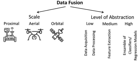
The most common categorization divides data fusion techniques into three groups^[9]: (a) raw data level (also denoted “low-level” and “early integration”), in which different types of data (raw or preprocessed) are simply concatenated into a single matrix, being used in cases in which pieces of data are of the same nature and were properly normalized. (b) Feature level (also denoted “mid-level” and “intermediate integration”), in which features are first extracted from different types of data and then concatenated into a matrix, being mostly used when pieces of data can be treated in such a way they generate features that are compatible and complementary. (c) Decision level (also denoted “high level” and “late integration”), in which classification and regression algorithms are applied separately to each type of datum and then the outputs generated by each model are combined, being more appropriate when data sources are too distinct to be combined at an earlier stage. An alternative classification of data fusion methods was proposed by Ouhami et al.^[10]: probability-based, evidence-based, and knowledge-based. Although both classifications are useful, the first one is more appropriate in the context of this work (Figure 1).

In the specific case of agriculture, data can be collected at three different scales—proximal, aerial, and orbital (satellites) (Figure 1). Applications that use proximal data include navigation systems for autonomous vehicles^{[11][12][13][14][15][16][17]}, fruit detection^{[18][19][20][21]}, plant disease detection^[22][23][24], delineation of homogeneous management zones^{[25][26][27][28][29]}, soil analysis^{[30][31][32][33][34][35][36]}, plant phenotyping^[37], among others. Aerial data (collected using UAVs) is used mostly for detection of certain objects (e.g., certain plant species and fruits)^[38] and for estimation of agricultural variables (e.g., soil moisture and nitrogen content)^[39][40][41]. Satellite data are used for mapping variables as diverse as soil moisture^[42][43][44], crop type^{[45][46][47][48][49][50]}, crop phenological states^[51][52], evapotranspiration^{[40][53][54][55][56][57][58]}, nitrogen status^{[59][60][61][62]}, biomass^[63][64], among others. While most data fusion approaches only use data in the same scale, a few studies have applied data originating from different scales ^{[10][26][28][31][38][40][51][52][64][65][66][67][68][69][70][71]}.

No.	Classes of Data Fusion Technique	No.	Classes of Data Being Fused
1	Regression methods	1	RGB images
2	STARFM-like statistical methods	2	Multispectral images
3	Geostatistical tools	3	Hyperspectral images
4	PCA and derivatives	4	Thermal images
5	Kalman filter	5	Laser scanning
6	Machine learning	6	SAR images
7	Deep learning	7	Spectroscopy
8	Decision rules	8	Fluorescence images
9	Majority rules	9	Soil measurements
10	Model output averaging	10	Environmental/weather measurements
11	Others	11	Inertial measurements
		12	Position measurements
		13	Topographic records and elevation models
		14	Historical data
		15	Others

2. Proximal Scale

The majority of studies dedicated to the proximal scale are concentrated in three main areas: prediction of soil properties, delineation of homogeneous zones, and robotic navigation and control. Applications, such as disease and fruit detection, prediction of water content and water stress, estimation of phonological state and yield prediction, are also present. Ten of the references also explored satellite data, and five studies combined proximal and aerial data. Data sources included cameras (RGB, multispectral, thermal, hyperspectral) spectrometers, conductance and resistivity sensors, GPS, inertial sensors, weather data, among many others. With such a variety of sensors available for field applications, efforts to explore their complementarities have been steadily growing (Table 2), but most problems still lack reliable solutions^[72].

Table 2. References considered in this study–proximal scale. L, M, and H mean low-, mid-, and high-level data fusion, respectively. The numbers in the fourth column are those adopted in Table 1 for each “fused data” class.

Ref.	Application	Fusion Technique	Fused Data	Mean Accuracy
[30]	Estimation of soil indices	SF (L), MOA (H)	7	0.80–0.90
[73]	Sustainable greenhouse management	Decision rules (L)	10	N/A
[72]	Human—robot interaction	LSTM-NN (L)	11	0.71–0.97
[25]	Delineation of homogeneous zones in viticulture	GAN (L), geostatistical tools (L)	2, 9	N/A
[26]	Delineation of homogeneous zones	Kriging and other geostatistical tools (L)	2, 9	N/A
[51]	Estimation of crop phenological states	Particle filter scheme (L)	2, 6, 10	0.93–0.96
[18]	Fruit detection	LPT (L) and fuzzy logic (L)	1, 4	0.80–0.95
[31]	In-field estimation of soil properties	RK (L), PLSR (L)	3, 9	>0.5
[74]	Delineation of homogeneous management zones	Kriging (L), Gaussian anamorphosis (L)	9, 15	0.66
[75]	Delineation of homogeneous management zones	Kriging (L), Gaussian anamorphosis (L)	9, 15	N/A
[27]	Delineation of homogeneous management zones	Kriging (L),Gaussian anamorphosis (L)	9, 15	N/A
[76]	Crop nutritional status determination	PCA (L)	7, 8	0.7–0.9
[22]	Detection of olive quick decline syndrome	CNN (M)	1	0.986
[65]	Monitoring Agricultural Terraces	Coregistering and information extraction (L/M)	5	N/A
[77]	Prediction of canopy water content of rice	BPNN (M), RF (M), PLSR (M)	2	0.98–1.00
[11]	Localization of a wheeled mobile robot	Dempster–Shafer (L) and Kalman filter (L)	11, 12	0.97
[19]	Immature green citrus fruit detection	Color-thermal probability algorithm (H)	1, 4	0.90–0.95
[28]	Delineation of management zones	K-means clustering (L)	2, 9, 14	N/A
[78]	Segmentation for targeted application of products	Discrete wavelets transform (M)	1	0.92
[12]	System for agricultural vehicle positioning	Kalman filter (L)	11, 12	N/A
[13]	System for agricultural vehicle positioning	Kalman filter (L)	11, 12	N/A
[67]	Yield gap attribution in maize	Empirical equations (L)	15	0.37–0.74
[32]	Soil environmental quality assessment	Analytic hierarchy process, weighted average (L)	15	N/A
[33]	Predict soil properties	PLSR (L)	7, 9, 13	0.80–0.96
[14]	System for agricultural vehicle positioning	Discrete Kalman filter (L)	11, 13	N/A
[34]	Estimating soil macronutrients	PLSR (L)	7, 9	0.70–0.95
[20]	Citrus fruit detection and localization	Daubechies wavelet transform (L)	1, 2	0.91
[15]	Estimation of agricultural equipment roll angle	Kalman filtering (L)	11	N/A
[79]	Predicting toxic elements in the soil	PLSR, PCA, and SPA (L/M)	7, 8	0.93–0.98
[68]	Review: image fusion technology in agriculture	N/A	N/A	N/A
[80]	Heterogeneous sensor data fusion	Deep multimodal encoder (L)	10	N/A
[81]	Agricultural vulnerability assessments	Binary relevance (L), RF (L), and XGBoost (L)	10,14	0.67–0.98
[35]	Prediction of multiple soil properties	SMLR (L), PLSR (L), PCA/SMLR combination (L)	7, 9	0.60–0.95
[82]	Prediction of environment variables	Sparse model (L), LR (L), SVM (L), ELM (L)	10	0.96
[64]	Estimation of biomass in grasslands	Simple quadratic combination (L)	2, 15	0.66–0.88
[23]	Plant disease detection	Kohonen self-organizing maps (M)	3, 8	0.95
[83]	Water stress detection	Least squares support vectors machine (M)	3, 8	0.99
[84]	Delineation of water holding capacity zones	ANN (L), MLR (L)	7, 9	0.94–0.97
[85]	Potential of site-specific seeding (potato)	PLSR (L)	2, 9	0.64–0.90
[86]	3D characterization of fruit trees	Pixel level mapping between the images (L)	4, 5	N/A
[87]	Measurements of sprayer boom movements	Summations of normalized measurements (L)	11	N/A
[10]	Review: IoT and data fusion for crop disease	N/A	N/A	N/A
[88]	Prediction of wheat yield and protein	Canonical powered partial least-squares (L)	7, 10	0.76–0.94
[69]	Wheat yield prediction	CP-ANN (L), XY-fused networks (L), SKN (L)	2, 7	0.82
[89]	Topsoil clay mapping	PLSR (L) and kNN (L)	7, 9, 13	0.94–0.96
[21]	Fruit detection	CNN (L); scoring system (H)	1, 2	0.84
[37]	3D reconstruction for agriculture phenotyping	Linear interpolation (L)	1, 10	N/A
[29]	Delineation of site-specific management zones	CoKriging (L)	2	0.55–0.77
[90]	Orchard mapping and mobile robot localization	Laser data projection onto the RGB images (L)	1, 5	0.97
[24]	Modelling crop disease severity	2 ANN architectures (L)	10, 15	0.90–0.98
[91]	Tropical soil fertility analysis	SVM (L), PLS (L), least squares modeling (L)	2, 8	0.30–0.95
[92]	Internet of things applied to agriculture	Hydra system (L/M/H)	9, 10, 15	0.93–0.99
[70]	Review: data fusion in agricultural systems	N/A	N/A	N/A
[36]	Soil health assessment	PLSR (L)	7, 9	0.78
[93]	Prediction of Soil Texture	SMLR (L), PLSR (L) and PCA (L)	7, 8	0.61–0.88
[94]	Rapid determination of soil class	Outer product analysis (L)	7	0.65
[16]	Navigation of autonomous vehicle	MSPI algorithm with Bayesian estimator (L)	11, 12	N/A
[38]	Detection of cotton plants	Discriminant analysis (M)	2, 7	0.97
[95]	Map-based variable-rate manure application	K-means clustering (L)	2, 9	0.60–0.93
[17]	Navigation of autonomous vehicles	Kalman filter (L)	11, 12	N/A
[96]	Robust tomato recognition for robotic harvesting	Wavelet transform (L)	1	0.93
[97]	Navigation of autonomous vehicle	Self-adaptive PCA, dynamic time warping (L)	1, 11	N/A
[98]	Recognition of wheat spikes	Gram–Schmidt fusion algorithm (L)	1, 2	0.60–0.79

 

3. Aerial Scale

Studies employing UAVs to solve agricultural problems are growing in number, but they are still outnumbered by proximal and orbital approaches. Most studies are dedicated to crop monitoring and object detection (weed, crops, etc.), although applications, such as phenotyping and water management, are also present. Almost all techniques are based on some kind of digital image (RGB, multispectral, thermal, hyperspectral). Many approaches explore the complementarity of aerial images with proximal (four articles) and orbital (six articles) data. Only eight studies employed the aerial data alone (Table 3).

Table 3. References considered in this study–aerial scale. L, M, and H mean low-, mid-, and high-level data fusion, respectively. The numbers in the fourth column are those adopted in Table 1 for each “fused data” class.

Ref.	Application	Fusion Technique	Fused Data	Mean Accuracy
[99]	Root zone soil moisture estimation	NN (M), DRF (M), GBM (M), GLM (M)	2,11	0.90–0.95
[100]	Gramineae weed detection in rice fields	Haar wavelet transformation (L)	1, 2	0.70–0.85
[65]	Monitoring agricultural terraces	Coregistering and information extraction (L)	5	N/A
[66]	Spectral–temporal response surfaces	Bayesian data imputation (L)	2, 3	0.77–0.83
[101]	Phenotyping of soybean	PLSR (L), SVR (L), ELR (L)	1, 2, 4	0.83–0.90
[39]	Soybean yield prediction	PLSR (M), RF (M), SVR (M), 2 types of DNN (M)	1, 2, 4	0.72
[52]	Crop monitoring	PLSR (M), RF (M), SVR (M), ELR (M)	1, 2	0.60–0.93
[40]	Evapotranspiration estimation	MSDF-ET (L)	1, 2, 4	0.68–0.77
[10]	Review: IoT and data fusion for crop disease	N/A	N/A	N/A
[102]	Arid and semi-arid land vegetation monitoring	Decision tree (L/M)	3, 5	0.84–0.89
[41]	Biomass and leaf nitrogen content in sugarcane	PCA and linear regression (L)	2, 5	0.57
[70]	Review: data fusion in agricultural systems	N/A	N/A	N/A
[103]	Navigation system for UAV	EKF (L)	11, 12	0.98
[38]	Detection of cotton plants	Discriminant analysis (M)	2	0.97
[71]	Vineyard monitoring	PLSR (M), SVR (M), RFR (M), ELR (M)	2	0.98

 

4. Orbital Scale

A large portion of the articles employing satellite images aimed to either compensate for data gaps present in a primary data source by fusing it with another source of data (for example, combining optical and SAR images)^{[6][45][47][48][49][51][104][105]}, or increase the spatial resolution of the relatively coarse images collected by satellites with high revisit frequencies^{[42][43][44][55][57][58][106][107][108][109]}. In the latter, the fused results usually inherit the details of the high spatial resolution images and the temporal revisit the frequencies of their counterparts, although the quality of the fused data usually do not match that obtained through actual missions, especially when surface changes are rapid and subtle^[110]. As argued by Tao et al.^[111], different sensors and image processing algorithms lead inevitably to data with some level of inconsistency, which can make rapid changes difficult to detect.

Landsat and MODIS images and products still dominate, but other satellite constellations, such as Sentinel, Worldview, GeoEye, and others, are being increasingly adopted. Data fusion has been applied to satellite images for quite some time, and well established techniques, such as STARFM and its variants, are still often used, but the interest for machine learning techniques, especially in the form of deep learning models, has been growing consistently. Water management in its several forms (evapotranspiration estimation, mapping of irrigated areas, drought detection, etc.) is by far the most common application. Yield estimation, crop monitoring, land cover classification, and prediction of soil properties are also common applications.

A major challenge associated with the orbital scale is the existence of highly heterogeneous regions with a high degree of fragmentation^[108][112]. Solutions to this problem are not trivial and, as stated by Masiza et al.^[113], “…successful mapping of a fragmented agricultural landscape is a function of objectively derived datasets, adapted to geographic context, and an informed optimization of mapping algorithms”. However, there are cases in which target areas can have sizes smaller than the pixel resolution of the satellite images^[53]. In theses cases, pairing the images with images or other types of data obtained at higher resolutions (aerial or proximal) may be the only viable solution. Satellite data were fused together with proximal and aerial data in ten and six studies, respectively (Table 4).

Table 4. References considered in this study–orbital scale. L, M, and H mean low-, mid-, and high-level data fusion, respectively. The numbers in the fourth column are those adopted in Table 1 for each “fused data” class.

Ref.	Application	Fusion Technique	Fused Data	Mean Accuracy
[42]	Soil moisture mapping	ESTARFM (L)	2	0.70–0.84
[45]	Crop type mapping	2D and 3D U-Net (L), SegNet (L), RF (L)	2, 6	0.91–0.99
[43]	Estimation of surface soil moisture	ESTARFM (L)	2	0.55–0.92
[26]	Delineation of homogeneous zones	Kriging and other geostatistical tools	2, 9	N/A
[51]	Estimation of crop phenological states	Particle filter scheme (L/M)	2, 6, 10	0.93–0.96
[53]	Evapotranspiration mapping at field scales	STARFM (L)	2	0.92–0.95
[31]	In-field estimation of soil properties	RK (L), PLSR (L)	3, 9	>0.5
[59]	Estimation of wheat grain nitrogen uptake	BK (L)	2, 3	N/A
[44]	Surface soil moisture monitoring	Linear regression analysis and Kriging (L/M)	2, 15	0.51–0.84
[46]	Crop discrimination and classification	Voting system (H)	2, 6	0.96
[9]	Review on multimodality and data fusion in RS	N/A	N/A	N/A
[47]	Crop Mapping	Pixelwise matching (H)	2, 6	0.94
[110]	Review on fusion between MODIS and Landsat	N/A	N/A	N/A
[106]	Mapping crop progress	STARFM (L)	2	0.54–0.86
[66]	Generation of spectral–-temporal response	Bayesian data imputation (L)	2, 3	0.77–0.83
[28]	Delineation of management zones	K-means clustering (L)	2, 9, 14	N/A
[114]	Mapping irrigated areas	Decision tree (L)	2	0.67–0.93
[54]	Evapotranspiration mapping	Empirical exploration of band relationships (L)	2, 4	0.20–0.97
[28]	Delineation of management zones	K-means clustering (L)	2, 9, 14	N/A
[67]	Yield gap attribution in maize	Empirical equations (L)	15	0.37–0.74
[63]	Change detection and biomass estimation in rice	Graph-based data fusion (L)	2	0.17–0.90
[107]	Leaf area index estimation	STARFM (L)	2	0.69–0.76
[55]	Evapotranspiration estimates	STARFM (M)	2	N/A
[115]	Classification of agriculture drought	Optimal weighting of individual indices (M)	2	0.80–0.92
[56]	Mapping daily evapotranspiration	STARFM (L)	2	N/A
[20]	Mapping of cropping cycles	STARFM (L)	2	0.88–0.91
[116]	Evapotranspiration partitioning at field scales	STARFM (L)	2	N/A
[68]	Review: image fusion technology in agriculture	N/A	N/A	N/A
[52]	Crop monitoring	PLSR (M), RF (M), SVR (M), ELR (M)	1, 2, 4	0.60–0.93
[113]	Mapping of smallholder crop farming	XGBoost (L/M and H), RF (H), SVM (H), ANN (H), NB (H)	2, 6	0.96–0.98
[64]	Estimation of biomass in grasslands	Simple quadratic combination (L/M)	2, 15	0.66–0.88
[40]	Evapotranspiration estimation	MSDF-ET (L)	1, 2, 4	0.68–0.77
[117]	Semantic segmentation of land types	Majority rule (H)	2	0.99
[118]	Eucalyptus trees identification	Fuzzy information fusion (L)	2	0.98
[10]	Review: IoT and data fusion for crop disease	N/A	N/A	N/A
[69]	Wheat yield prediction	CP-ANN (M), XY-fused networks (M), SKN (M)	2, 7	0.82
[112]	Drought monitoring	RF (M)	2, 15	0.29–0.77
[48]	Crop type classification and mapping	RF (L)	2, 6, 13	0.37–0.94
[119]	Time series data fusion	Environmental data acquisition module	10	N/A
[57]	Evapotranspiration prediction in vineyard	STARFM (L)	2	0.77–0.81
[108]	Daily NDVI product at a 30-m spatial resolution	GKSFM (M)	2	0.88
[49]	Crop classification	Committee of MLPs (L)	2, 6	0.65–0.99
[6]	Multisource classification of remotely sensed data	Bayesian formulation (L)	2, 6	0.74
[111]	Fractional vegetation cover estimation	Data fusion and vegetation growth models (L)	2	0.83–0.95
[120]	Land cover monitoring	FARMA (L)	2, 6	N/A
[121]	Crop ensemble classification	mosaicking (L), classifier majority voting (H)	2	0.82–0.85
[70]	Review: data fusion in agricultural systems	N/A	N/A	N/A
[50]	In-season mapping of crop type	Classification tree (M)	2	0.93–0.99
[122]	Building frequent landsat-like imagery	STARFM (L)	2	0.63–0.99
[58]	Evapotranspiration mapping	SADFAET (M)	2	N/A
[123]	Temporal land use mapping	Dynamic decision tree (M)	2	0.86–0.96
[124]	High-resolution leaf area index estimation	STDFA (L)	2	0.98
[125]	Monitoring cotton root rot	ISTDFA (M)	2	0.79–0.97
[109]	Monitoring crop water content	Modified STARFM (L)	2	0.44–0.85
[104]	Soil moisture content estimation	Vector concatenation, followed by ANN (M)	2, 6	0.39–0.93
[126]	Impact of tile drainage on evapotranspiration	STARFM (L)	2	0.23–0.91
[127]	Estimation of leaf area index	CACAO method (L)	2	0.88
[105]	Mapping winter wheat in urban region	SVM (M), RF (M)	2, 6	0.98
[128]	Leaf area index estimation	ESTARFM (L), linear regression model (M)	2	0.37–0.95
[71]	Vineyard monitoring	PLSR (M), SVR (M), RFR (M), ELR (M)	2	0.98

Another important challenge is the difficulty of obtaining/collecting reference data for validation of the techniques applied. This problem can be particularly difficult if the reference data need to be gathered in-loco. It is also important to consider that, even if reference data can be collected, differences in granularity and the positions of the sample points can make the comparison with the fused data difficult or even unfeasible^[112].