2. Statistical Analysis
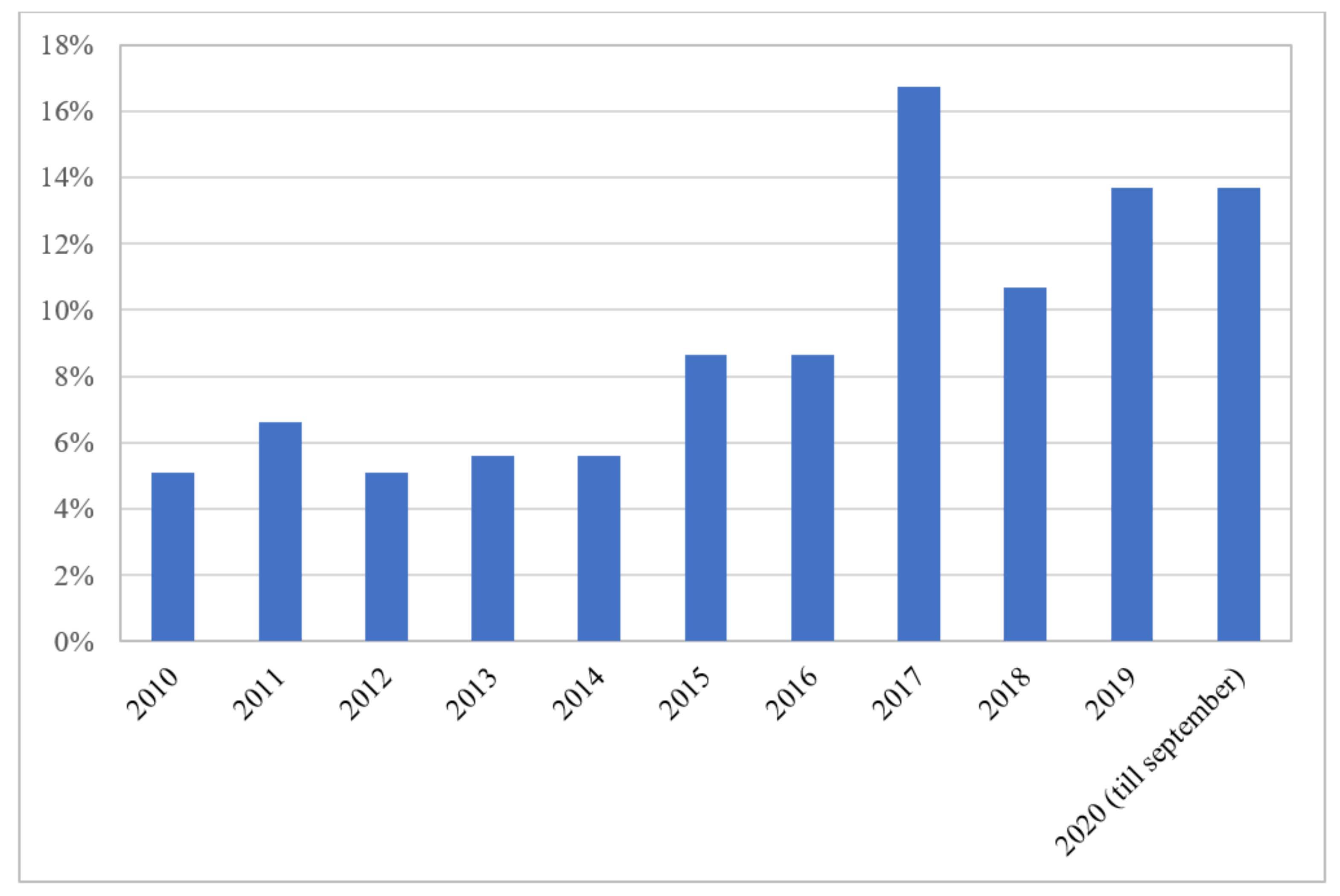
The number of research articles using machine learning (ML) to predict groundwater characteristics is growing after 2014 (Figure 1), with a spike in 2017. Out of 197 articles included for meta-analysis, 33 (16.75%) were published in 2017.
Figure 1. Number of research records included in the systematic review based on their date of publication.
Included records were published in various journals, of which the Journal of Hydrology (10.66%) published the largest set of papers, followed by Water Resources Management (7.11%), and Environmental Earth Sciences (5.08%).
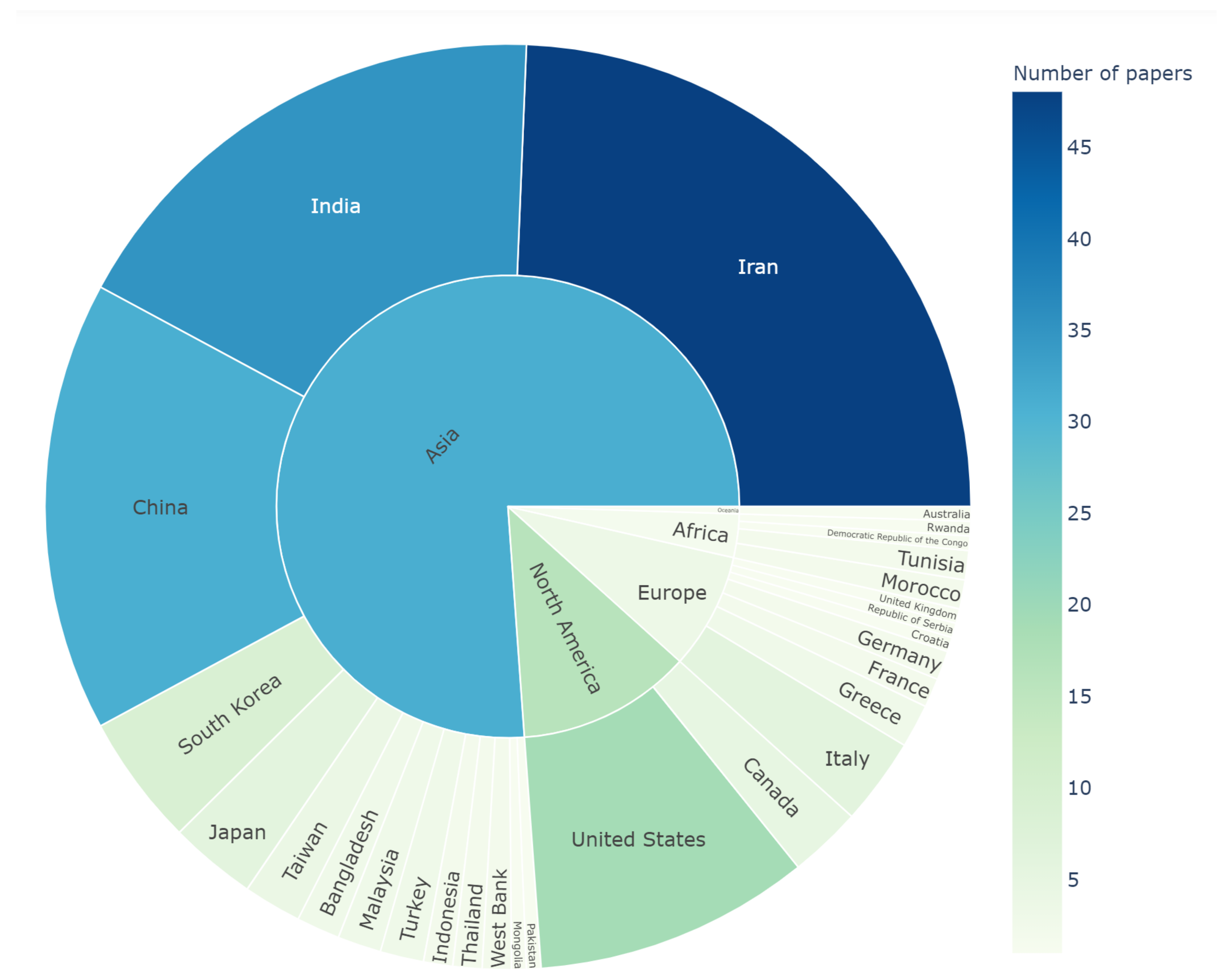
The systematic literature search showed that Iran (24%), India (18%), China (16%), and the United States (10%) had the highest number of articles, respectively (
Figure 2). Iran as the leading country in the number of articles in this systematic review also deals with a state of water bankruptcy partly due to anthropogenic depletion of its aquifers (Noori et al., 2021). The list of countries with the highest number of articles also agrees well with the list of countries with the highest dependency on groundwater resources. According to
[28], the top five nations with the largest estimated annual groundwater extractions in 2010 are India (251.00 km
3/year), China (111.95 km
3/year), the United States (111.70 km
3/year), Pakistan (64.82 km
3/year), and Iran (63.40 km
3/year). It is worth mentioning that Iran, India, China, and the United States use 87%, 89%, 54%, 71% of their groundwater extraction for irrigation, respectively (Margat and Van der Gun, 2013). It should be noted that groundwater depletion due to overdraft for mainly irrigation purposes is reported as a worldwide problem. According to the findings of
[29][30], Iran, India, China, and United states are among the countries with the most reliance on groundwater resources for food production and deal with the consequences of overdraft. Our findings reveal that the hotspots of groundwater consumption and depletion are the popular case studies for the application of ML in groundwater modeling and prediction. In total, the included articles in this study were from 28 countries (
Figure 2).
Figure 2. Pie chart of the included research articles based on the country of origin.
Most of the papers (56%) had a case study with an area less than 1000 km
2, followed by study areas between 1000 km
2 and 2000 km
2 (22%), and the remaining 23% had a case study with an area of more than 2000 km
2. Only 6% of the articles studied a confined aquifer, while 5% had a semi-confined aquifer and 89% had worked on an unconfined aquifer or did not mention the type of aquifer in their manuscript. Twenty-seven percent of the articles studied coastal aquifers and the remaining (73%) had a non-coastal aquifer as their case study. Being prone to seawater intrusion, groundwater salinization is a common problem in coastal aquifers, particularly where excessive groundwater pumping induces a decrease in the piezometric head
[31], and therefore, some of the reviewed studies had focused on predicting groundwater salinity in coastal aquifers
[32][33].
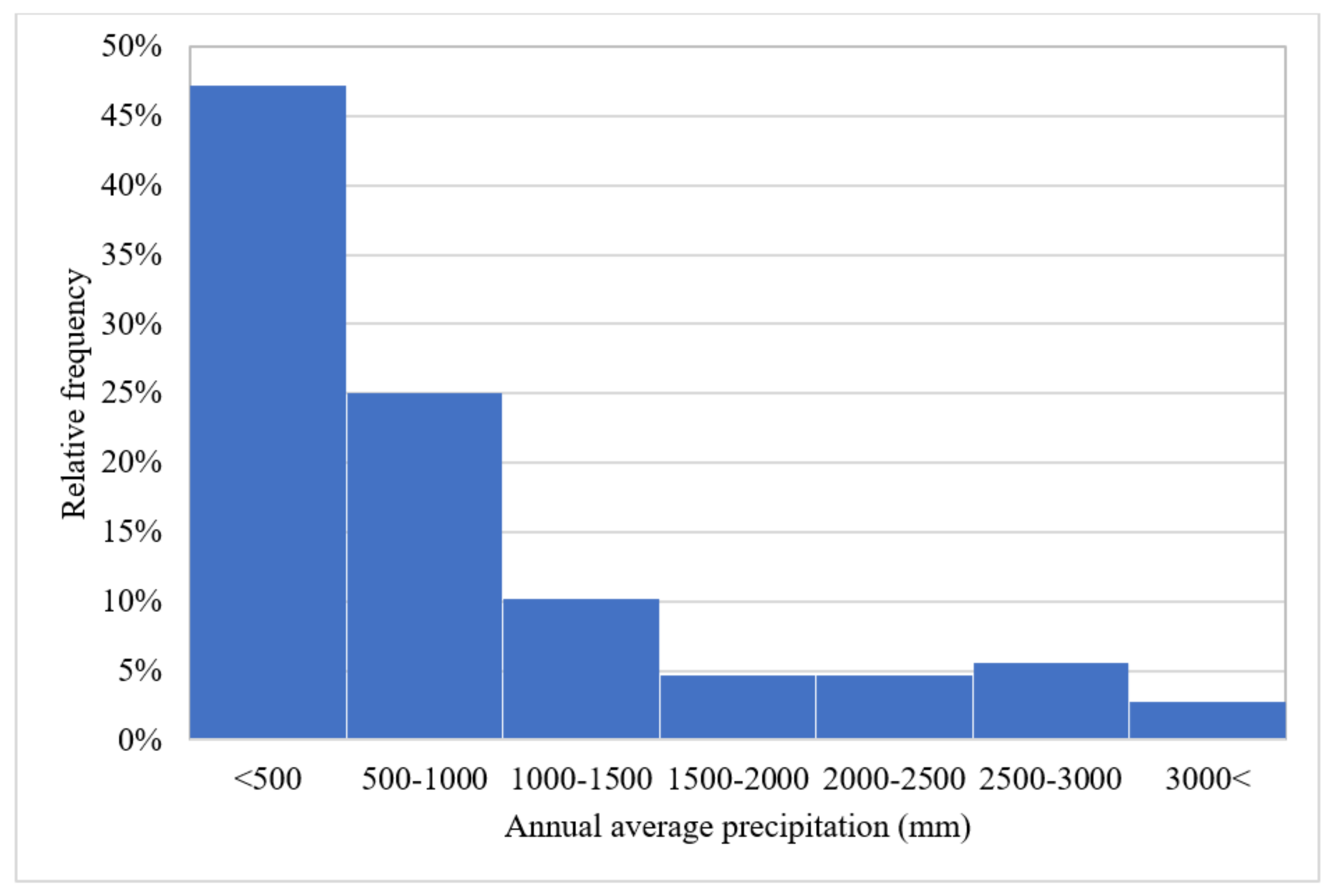
As shown in
Figure 3, a high percentage of the reviewed articles are from arid and semi-arid regions of the world, where surface water resources are generally scarce and highly unreliable
[34]. Moving from arid to humid regions, the reliability of surface water resources increases and, as a result, the interest in studying groundwater resources decreases (
Figure 3).
Figure 3. Reviewed articles’ proportion according to the average annual precipitation of their case studies.
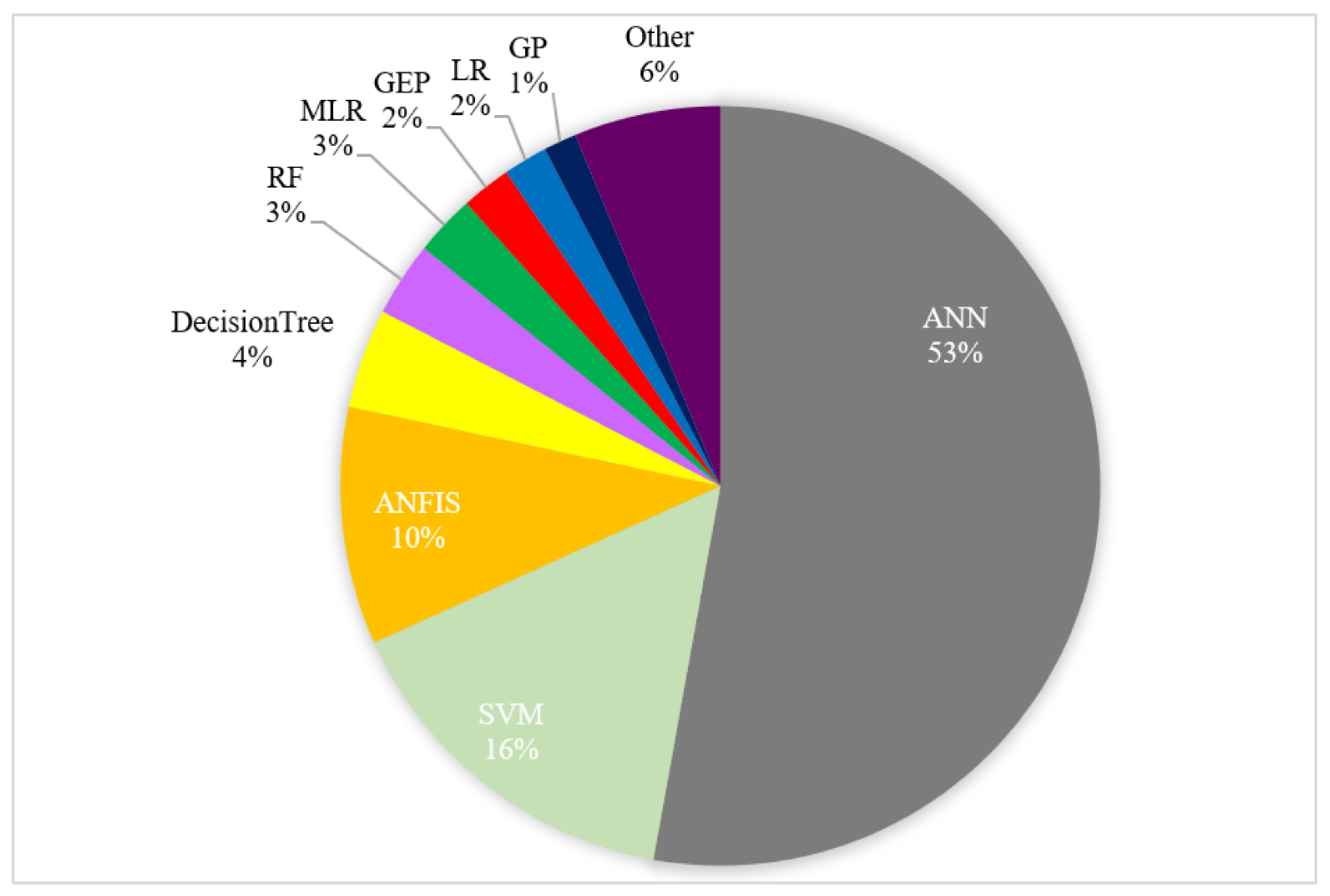
In total, 26 different ML methods were reported in the articles as tools to predict various characteristics of groundwater resources. Among them, ANN, SVM, and ANFIS were the most popular methods with 53%, 16%, and 10% of total records, while GEP, LR, and GP were applied much less (Figure 4).
Figure 4. The proportion of the reports according to the ML method that they have employed.
The employed ANN models had different architectures, but FFNN was the most used (around 66% of records), followed by NARX with 11.3% of records. Gradient descent (64.3%), LMA (19.5%), and PSO (5%) were the most used optimization algorithms for training ANN models. Most of the papers that used gradient descent mentioned using back-propagation for calculating gradients for the weights of the network. Seventy-nine records used wavelet transformation along with ML models, where 54.4%, 13.9%, and 10.1% of them utilized ANN, ANFIS, SVM models, respectively. According to the studies that used wavelet transformation, determining the appropriate decomposition level is an important step as it affects the ML models’ performance
[35][36]. Moosavi et al. (2013) suggest considering the periodicity and seasonality of data series to determine the appropriate number of decomposition levels. In summary, our meta-analysis shows that FFNN with gradient descent as an optimization algorithm is the most employed ML model to predict characteristics of groundwater resources. Based on its wide use and acceptable performance, it can be inferred that this model structure is a suitable choice for the prediction of groundwater characteristics.
Sample division into training, validation, and test sets is one of the important factors in designing ML models. Although some researchers divided the data into only training-testing subsets, using three subsets as training, validation, and testing is generally preferable. In the latter scenario, the testing set is never used in the process of model building while the validation set helps with the fine-tuning of the model hyperparameters and even choosing the best model structure. This procedure eliminates the risk of over-fitting (i.e., where an ML model will “memorize” the features of the training input data instead of actual “learning”) and ends up with more reliable results where the ML model shows its generality to work well with new, unseen data.
Cross-validation is another model validation technique that uses a resampling procedure and is especially useful when the sample data are limited. In the cross-validation process, instead of a fixed test set, input data are divided into some “folds” and in each training step, one fold is held out as the test set and the model is trained with the remaining data. After training the model, its performance is measured on the unseen test set (i.e., the held-out fold). This process repeats k times, where k is the number of folds, and at the end, the average of k measures of performance is reported as the final measure of model fitness. According to our meta-analysis, 16.2% of the articles used cross-validation, while 12.4% of records used both cross-validation and sample division strategies. A 96.2% of the articles divided their dataset into subsets, while around 80% of these articles only had train-test subsets and 20% had three subsets division. From a data science point of view, this can be a weakness, especially if the models have been exposed to the validation data before the final model evaluation.
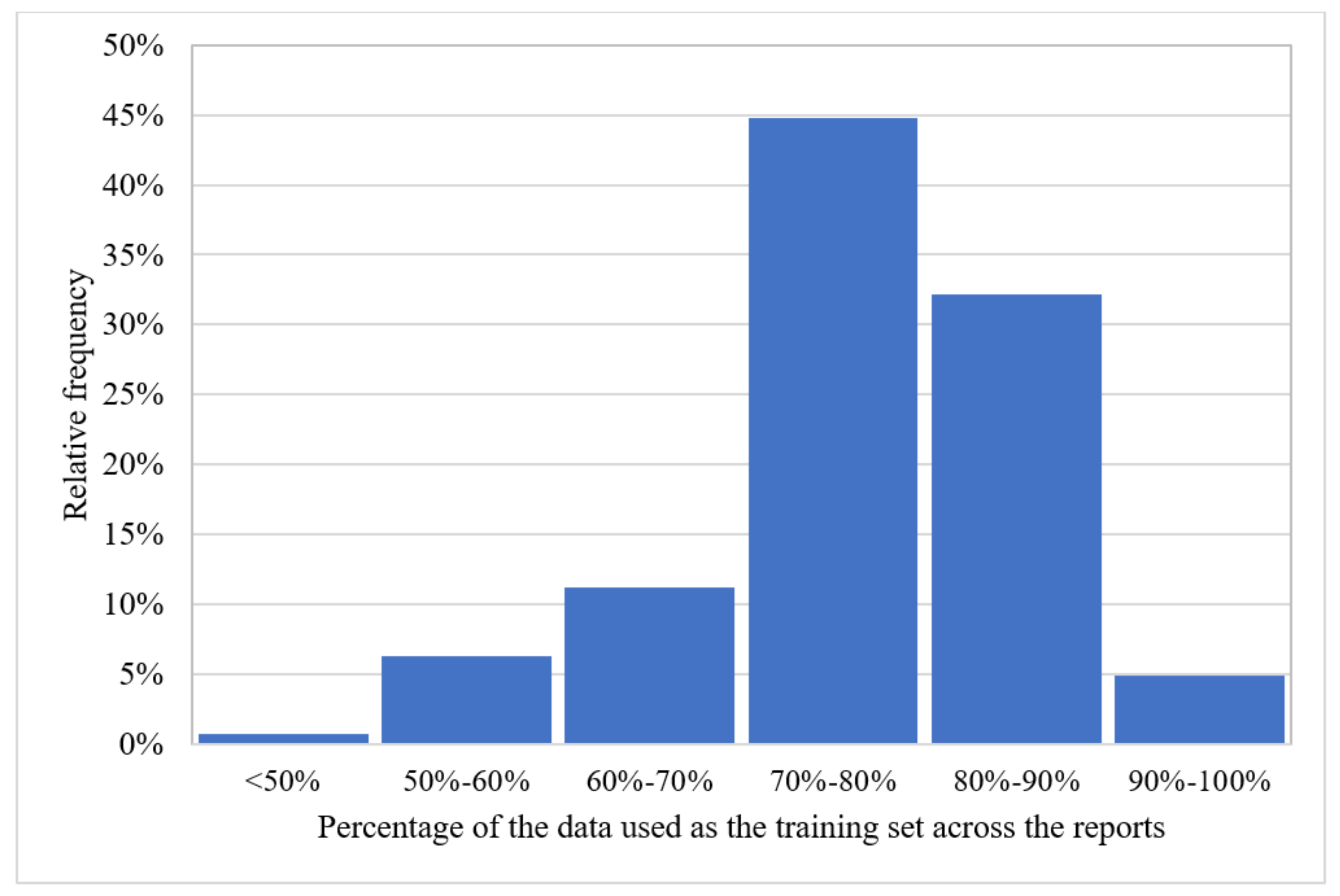
As shown in Figure 5, most of the articles have used 70–80% of the data as the training subset and the remaining as the test subset. Similarly, most of the articles having three subsets have used 60–70% of the data as the train set and divided the remaining into validation and test sets.
Figure 5. The proportion of articles dividing the data into two training-testing subsets.
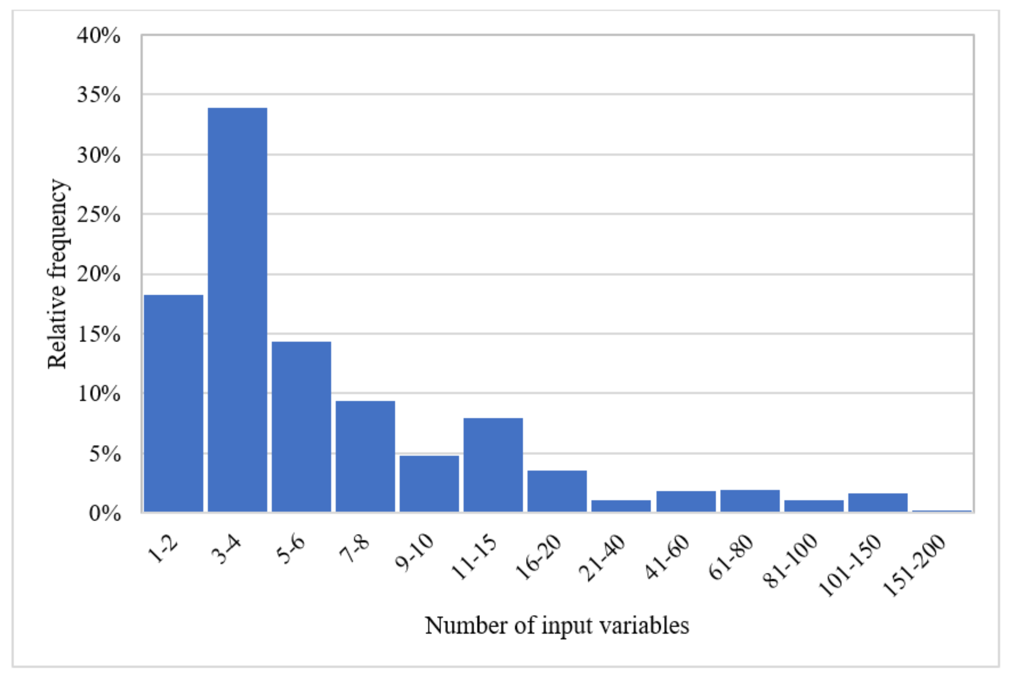
The input data length, temporal resolution, and the number of categories are other important factors in ML modeling in general and particularly in hydrological studies. To train a reliable data-driven model in groundwater studies, the model needs to be fed with temporally inclusive input data to be able to predict variable geohydrological conditions and to learn the seasonality. As depicted in Figure 6, while most of the articles had lower than 8 input categories, a considerable portion had between 3 to 4 input categories. This might have two main reasons; first, in many case studies, many potential variables are poorly measured, and secondly, increasing the number of input variables would cause some unfavorable phenomenon in modeling such as the curse of dimensionality. Additionally, the use of fewer input variables to training ML models can imply the efficacy of these models in predicting groundwater characteristics. This is especially important in ungauged regions. The use of ML models in these regions can also be favorable from an economic point of view since these regions usually rely on agriculture, and an accurate estimation of, for example, the groundwater level using limited input data can assist with more cost-efficient irrigation scheduling.
Figure 6. The proportion of articles according to their number of inputs.
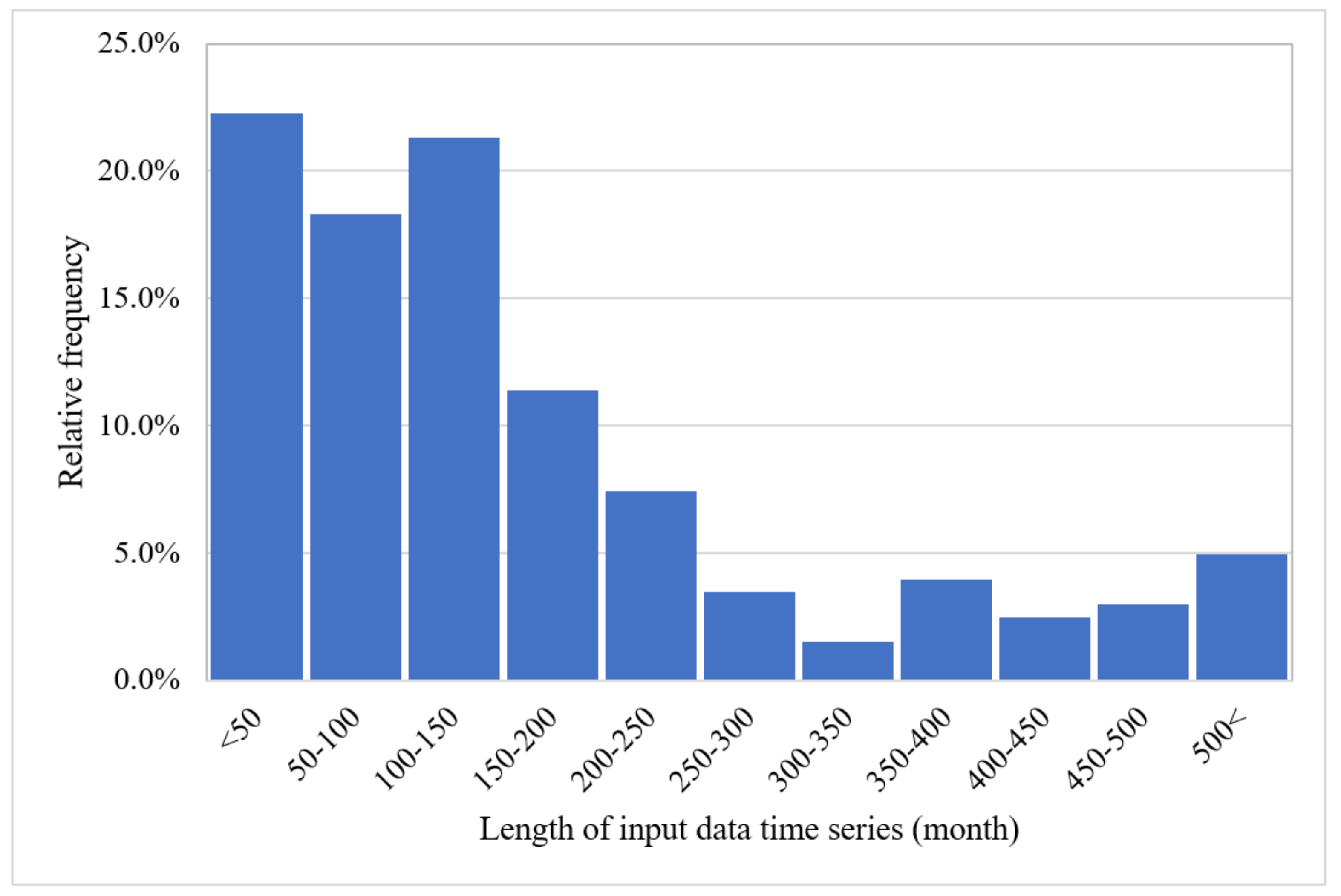
As shown in Figure 7, the length of the input data time series was mostly up to around 12 years, and rarely more than 20 years, with very few studies having more than 40 years of input data to train the ML models.
Figure 7. Percentage of the reviewed articles according to the length of the input data time series.
The monthly temporal resolution was by far the most popular among the articles (around 65% of the records), followed by the daily resolution with 19.6%. This could imply a higher availability of groundwater data in the monthly temporal resolution more than other resolutions. Furthermore, the monthly resolution might be more favorable for large-scale water managing stakeholders and policymakers.
Although our research question was not limited to any specific characteristic, researchers found that most of the research articles using ML algorithms in groundwater studies were focused on the prediction of the groundwater level (82.5%). The possible explanation for this large number might be related to denser measurements of the groundwater level compared to other variables in practice. Moreover, the groundwater level is a continuous variable that could be regionalized through various interpolation methods. In total, 17 groundwater characteristics were found in the reviewed articles to be predicted using ML, with a discharge or baseflow (6.1%), groundwater recharge (2.7%), and freshwater-saltwater interface level (2.5%) being the most popular ones after groundwater level (Table 1). Our analysis shows that the most adopted input variables for training ML models to predict the groundwater level were groundwater levels at earlier time steps (26.7%), precipitation (25.1%), temperature (13.6%), and evaporation or evapotranspiration (10.5%). Humidity or moisture (2.2%), river discharge (1.9%), surface runoff (1.8%), pumping data (1.7%), and river stage (1.6%) were other important input variables.
Table 1. Groundwater characteristics predicted by ML models in the reviewed articles.
| Predicted Variable |
Percentage of Reports |
| Groundwater level |
82.5% |
| Discharge |
6.1% |
| Groundwater recharge |
2.7% |
| Freshwater–saltwater interface level |
2.5% |
| Salinity |
1.3% |
| Groundwater level fluctuation |
1.4% |
| Total dissolved solids |
0.6% |
| Electrical conductivity |
0.6% |
| Aquifer loss coefficient |
0.5% |
| Fluoride |
0.5% |
| Sodium adsorption ratio |
0.4% |
| Nitrate nitrogen (NO3-N) |
0.2% |
| Contamination level |
0.2% |
| Sulfate (SO4) |
0.2% |
| Hydraulic head change |
0.1% |
| Dissolved oxygen |
0.1% |
| Groundwater storage variation |
0.1% |
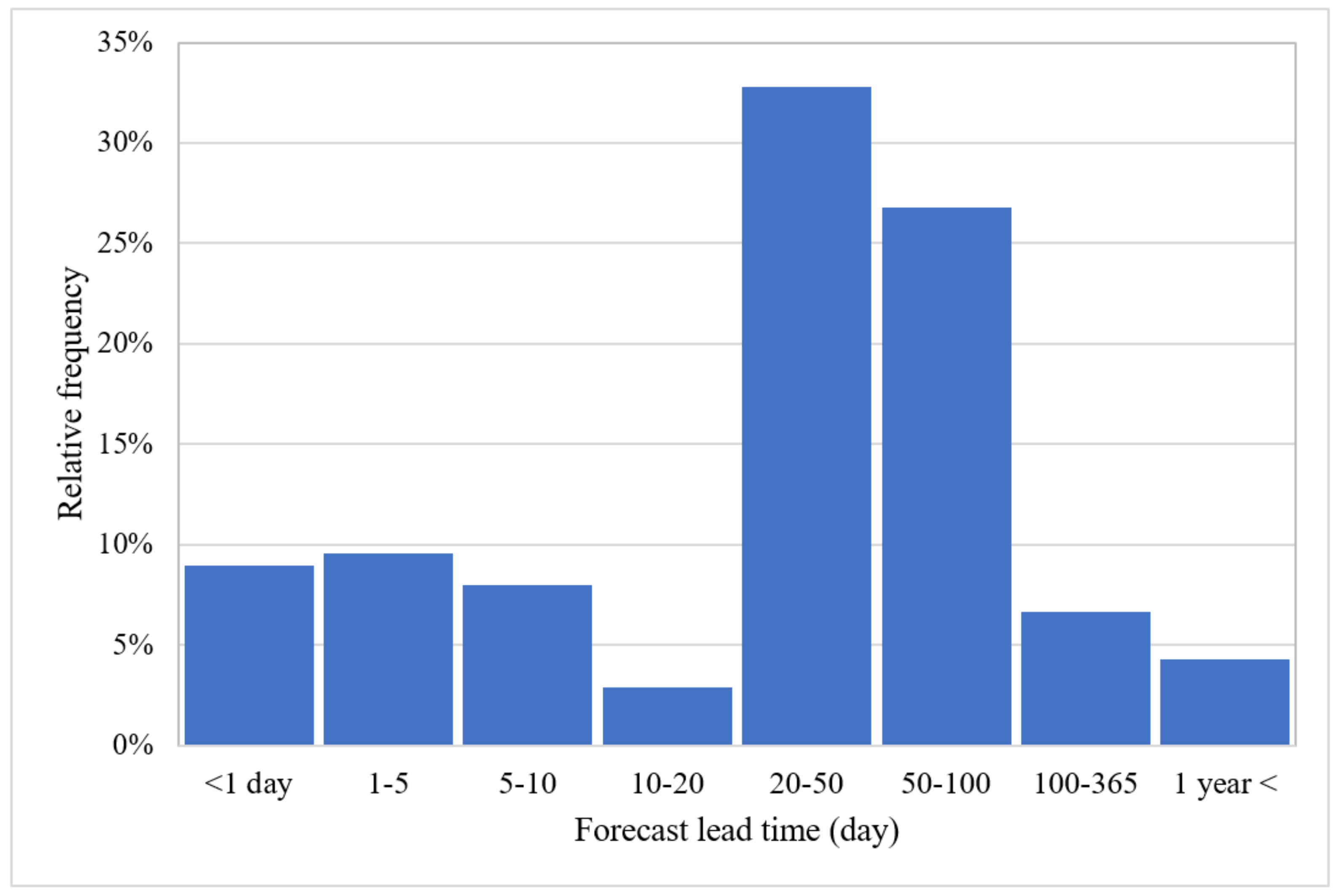
Around 40% of the reports have used input variable selection techniques to determine what variables should be included in the ML model based on their importance. Cross-correlation analysis (36.2%), autocorrelation analysis (19.9%), and partial autocorrelation function (17.1%) were the most adopted techniques. After training the ML model, 61.3% of the reviewed articles used their model to forecast future states of groundwater resources. Figure 8 shows the relative frequency of the forecast timespan.
Figure 8. Percentage of reports according to their forecast periods.
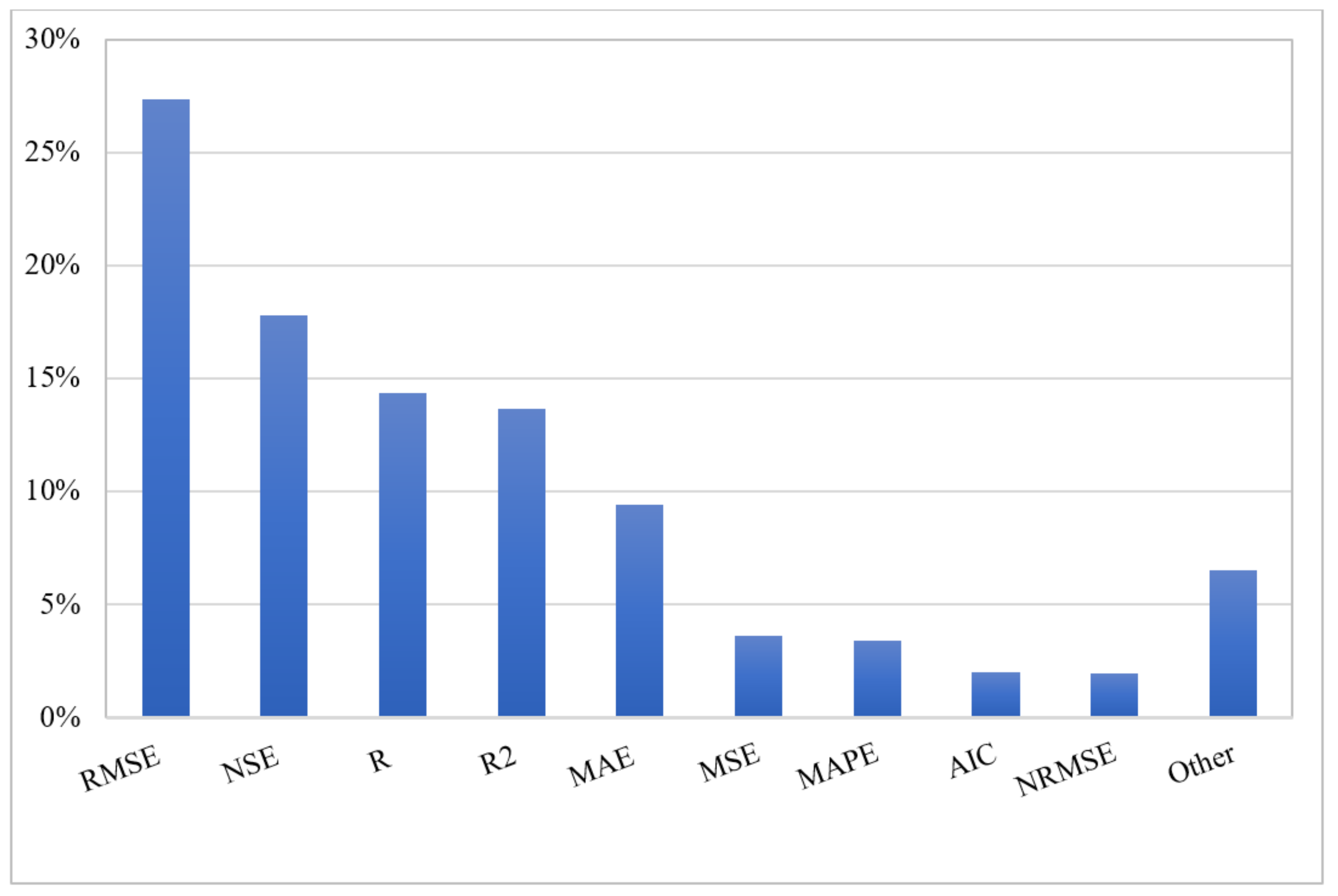
Figure 9 presents the percentage of statistical indicators used to measure the accuracy of the ML model of the groundwater level. RMSE (27.4%), NSE (17.8%), the correlation coefficient (14.3%), coefficient of determination (13.7%), and MAE (9.4%) were the most popular measures of performance. RMSE is also the most adopted measure of performance for other predicted characteristics. RMSE indicates the absolute fit of the model to the data and is a suitable measure of performance with the same units as the predicted variable. On the other hand, the coefficient of determination (R2) is a relative measure and does not indicate the absolute precision of the model.
Figure 9. The proportion of employed quantitative measures of performance.
3. Meta-Analysis
As mentioned earlier, more than 82% of reviewed articles had used ML models to predict the groundwater level and only around 18% of articles were focused on other groundwater characteristics. As a result, our meta-analysis is mostly focused on groundwater level forecasting. Researchers also presented the outcome of the meta-analysis for other characteristics, where possible. Here, they used violin plots that show the probability density of the data at different values using a rotated kernel density plot, which provides insights into the distribution of data and facilitates data analysis and exploration
[37][38]. In all violin plots, the red dot shows the mean, while the box demonstrates the first, second and third quartiles, where the middle bar is the median.
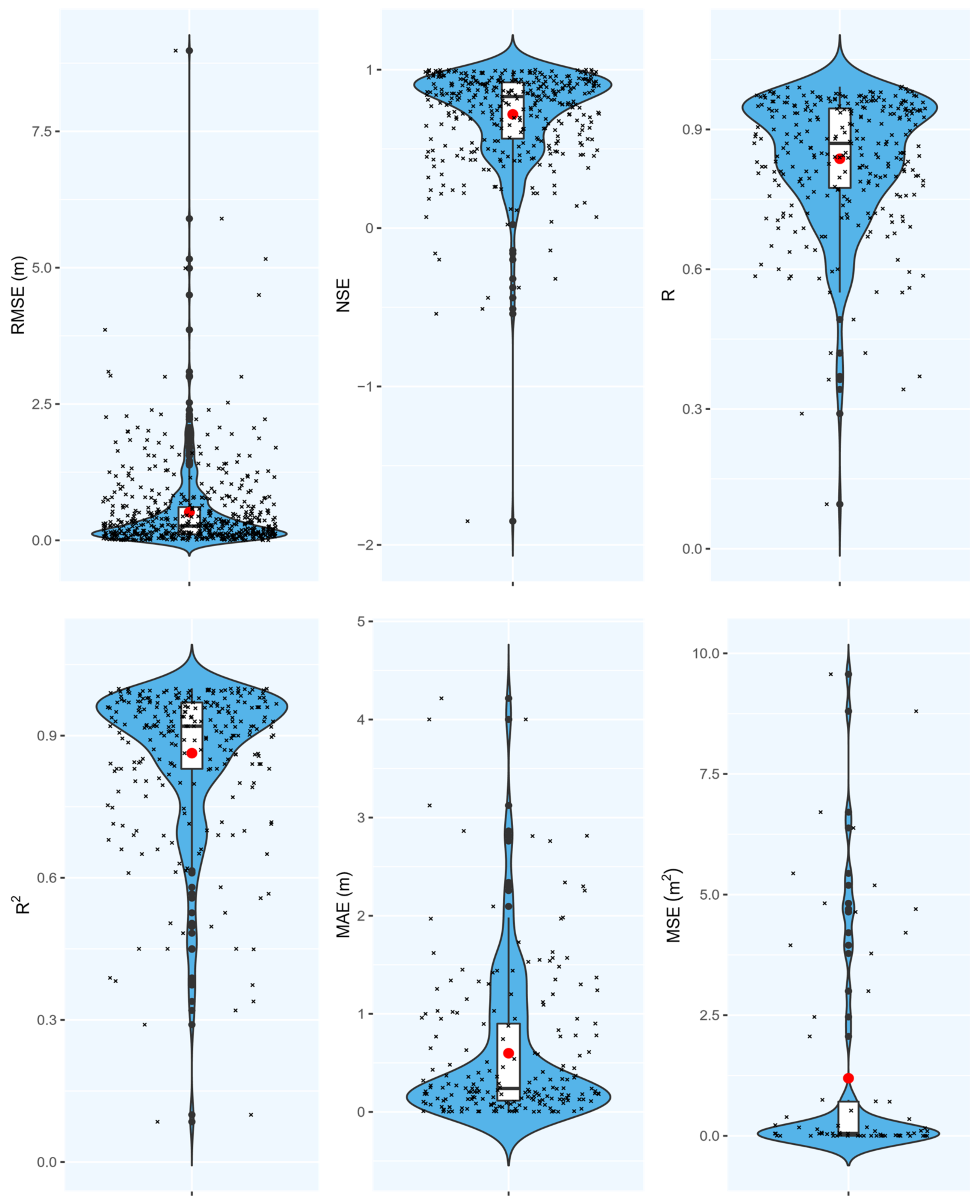
Figure 10 shows the results of the meta-analysis on the predictive capability of ML models for groundwater level prediction through various measures of performance.
Figure 10. Quantitative measures of performance for ML models predicting groundwater levels.
For instance, 546 records with an RMSE performance were used to construct the violin plot of RMSE in Figure 10 (mean RMSE of 0.52 m). It should be noted that different papers had various case studies with distinct groundwater levels, therefore, comparing RMSEs might lead to misleading results in some cases. In other words, the variation of the groundwater level in a shallow aquifer is inherently different from that of a deep aquifer. As shown in Figure 10, the results of R2 presented from 270 records are promising.
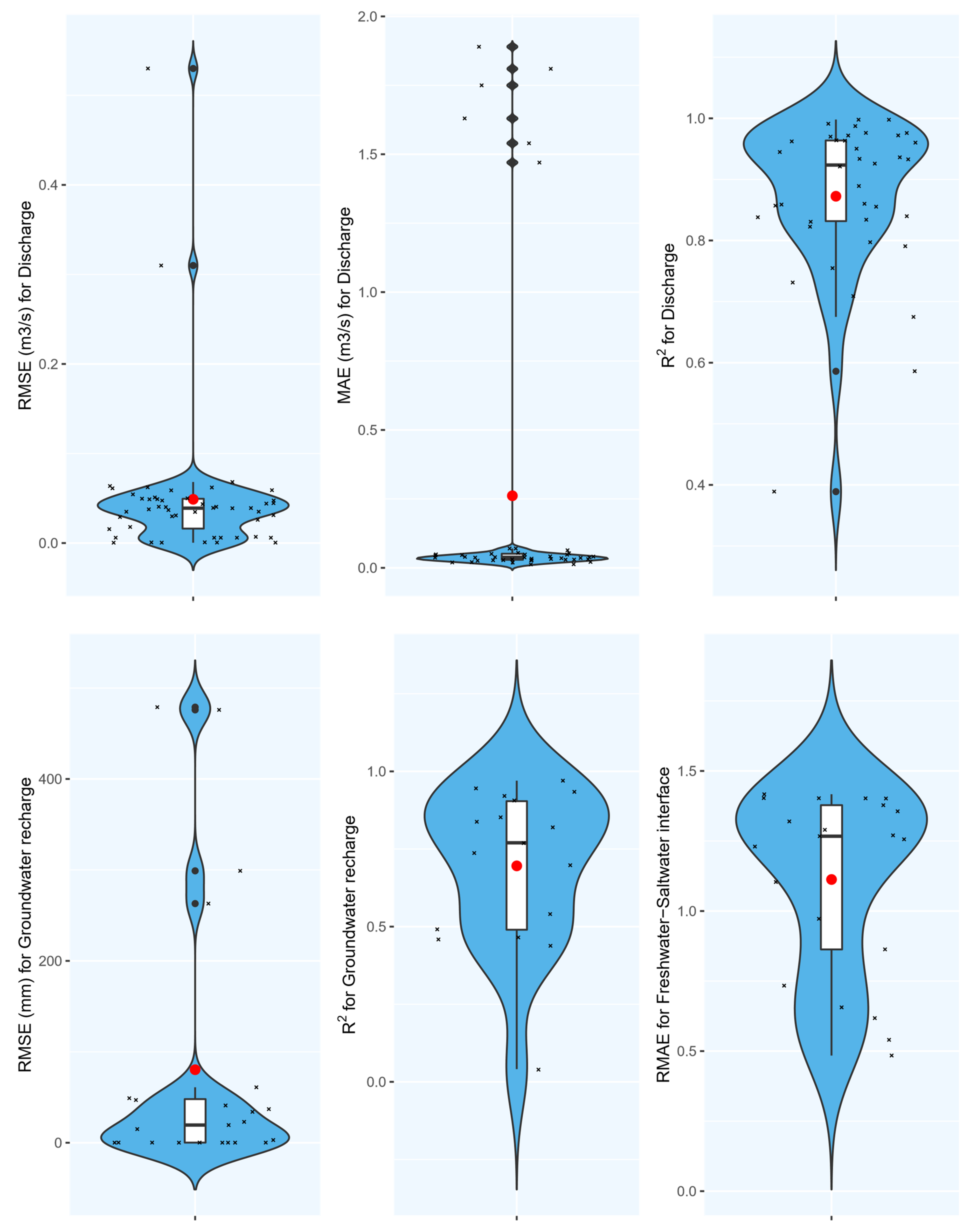
Figure 11 illustrates the results for other characteristics that had enough records (more than 15) to conduct a meta-analysis. These violin plots show an acceptable accuracy of ML models to predict a variety of groundwater characteristics. Contrary to the groundwater level prediction (Figure 11), these results are from fewer records, therefore, general conclusions should be drawn with caution. What is obvious, however, is the potential of data-driven models to estimate miscellaneous groundwater characteristics accurately with a lower number of input data and easier model structures compared to physical models.
Figure 11. Results of meta-analysis for various groundwater characteristics.
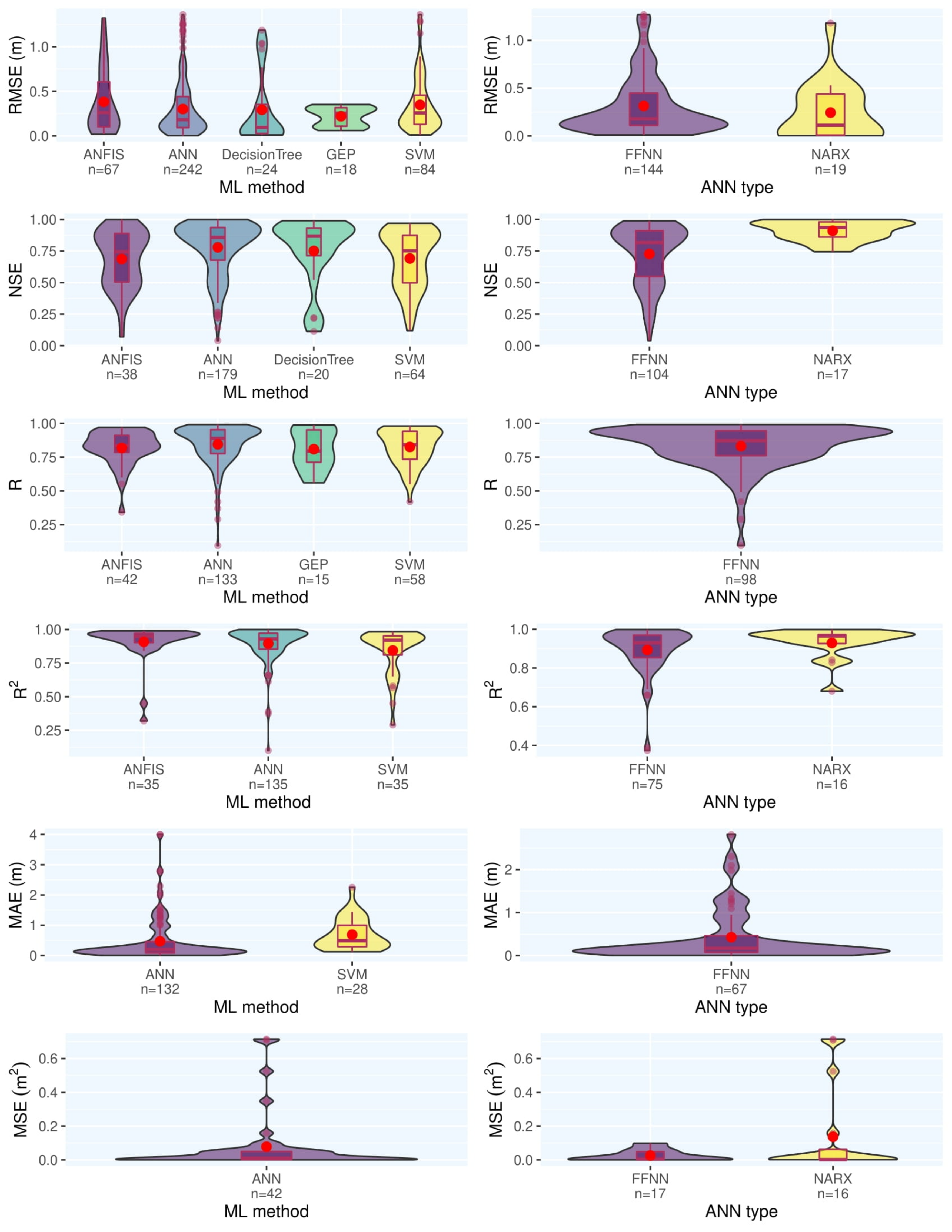
Along with a one-dimensional meta-analysis on the capability of the ML models to predict groundwater characteristics, researchers categorized the reviewed papers’ reports based on different criteria to cast light on the different aspects of data-driven modeling in groundwater studies. Figure 12 represents the results for different ML methods and ANN architectures with a threshold of 15 records in each category. Most employed ML methods (e.g., ANFIS, ANN, SVM) have a comparable and even similar performance according to reported statistical measures. However, ANN slightly outperforms other models in most cases. Generally, it can be inferred that the most influencing factor in the performance of ML models in groundwater studies is the quality and quantity of the input data and not the model. Comparing different ANN architectures, they see that NARX outperforms FFNN, but due to the much lower number of records for NARX, this finding is not conclusive, and more investigation is required.
Figure 12. Results of meta-analysis for ML models and ANN architectures to predict groundwater level.
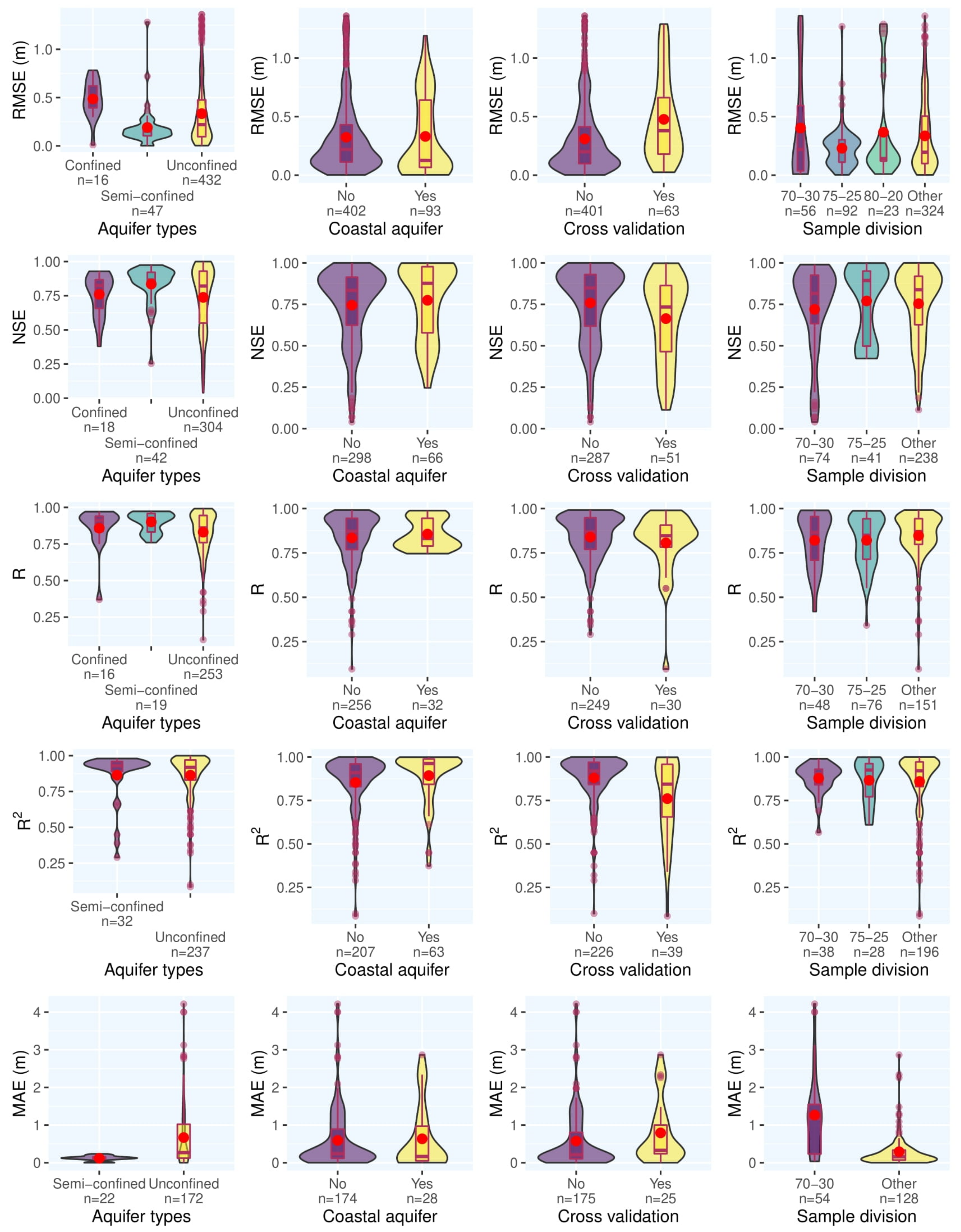
Figure 13 contrasts the results for the type of the aquifer, whether the aquifer is coastal or not, whether cross-validation is used or not, and various schemes for sample division. As researchers can see in Figure 13, results from different aquifer types are comparable and no obvious trend can be found. Although the number of records is different for coastal and non-coastal aquifers, from Figure 13 they can infer that the model results for the coastal aquifers are slightly superior. Moreover, Figure 13 shows that in the case of sample division without cross-validation, models are working slightly better. This might be because in cross-validation the considered dataset is divided into different training and test sets multiple times, and the total performance of a model would be the average of all individual performances; however, in classical validation, there is only one training and one test set. Therefore, even one subset with a low performance would decrease the total performance in the cross-validation technique. There is no meaningful trend in the results for different sample division proportions.
Figure 13. Meta-analysis results according to various subcategories in the reviewed reports.
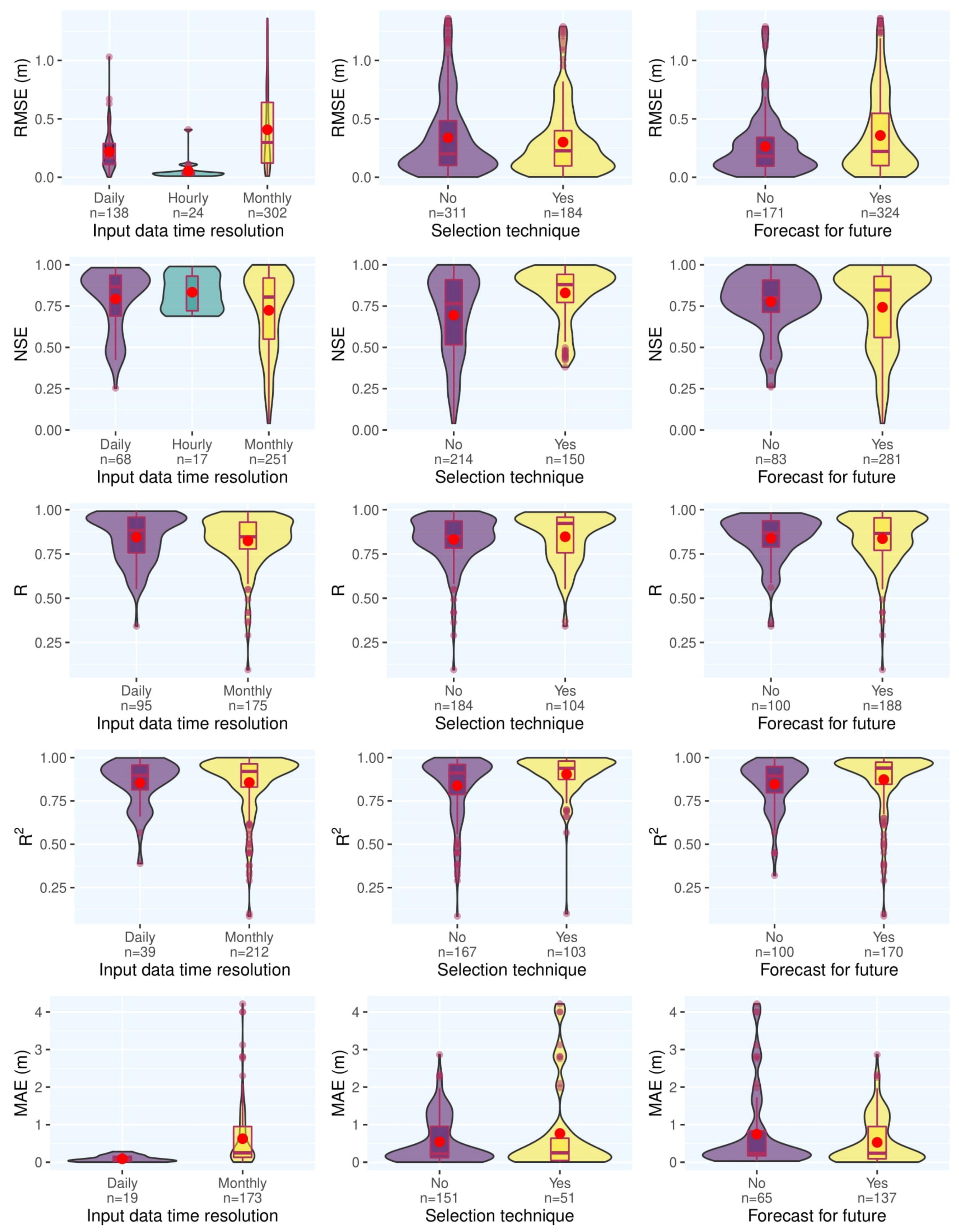
Figure 14 shows the outcome of meta-analysis for input data’s temporal resolution, the input variable selection technique, and forecast for the future. The daily time series is marginally better than the monthly time series in terms of model accuracy. Studies that used input variable selection techniques had superior results to those without these techniques. It can be inferred that input variable selection is a useful step in setting up ML models to predict groundwater characteristics. According to Figure 14, there is no meaningful trend in the results comparing papers that do forecast for the future and papers that do not.
Figure 14. Meta-analysis results for three subcategories in the reviewed reports for groundwater level prediction.