Your browser does not fully support modern features. Please upgrade for a smoother experience.
Please note this is an old version of this entry, which may differ significantly from the current revision.
Subjects:
Area Studies
Elastic modulus (E) is a key parameter in predicting the ability of a material to withstand pressure and plays a critical role in the design of rock engineering projects. E has broad applications in the stability of structures in mining, petroleum, geotechnical engineering, etc. E can be determined directly by conducting laboratory tests, which are time consuming, and require high-quality core samples and costly modern instruments. Thus, devising an indirect estimation method of E has promising prospects.
- elastic modulus
- K-fold cross-validation
- mining
1. Introduction
Elastic modulus (E) is a key parameter in predicting the ability of a material to withstand pressure and plays a critical role in the design process of rock-related projects. E has broad applications in the stability of structures in mining, petroleum, geotechnical engineering, etc. Accurate estimation of deformation properties of rocks, such as E, is very important for the design process of any underground rock excavation project. Intelligent indirect techniques for designing and excavating underground structures make use of a limited amount of data for design, saving time and money while ensuring the stability of the structures. This study has economic and even social implications, which are integral elements of sustainability. Moreover, this paper aims to determine the stability of underground mine excavation, which may otherwise result in a disturbed overlying aquifer and earth surface profile, adversely affecting the environment. E provides insight into the magnitude and characteristics of the rock mass deformation due to changes in the stress field. Deformation and behavior of different types of rocks have been examined by different scholars [1,2,3,4]. Usually, there are two common methods, namely, direct (destructive) and indirect (non-destructive), to calculate the strength and deformation of rocks. Based on the principles suggested by ISRM (International Society for Rock Mechanics) and the ASTM (American Society for Testing Materials), direct evaluation of E in the laboratory is a complex, laborious, and costly process. Simultaneously, in the case of fragile, internally broken, thin, and highly foliated rocks, the preparation of a sample is very challenging [5]. Therefore, attention should be given to evaluate E indirectly by the use of rock index tests.
Several authors have developed prediction frameworks to overcome these limitations by using machine learning (ML)-based intelligent approaches such as multiple regression analysis (MRA), artificial neural network (ANN), and other ML methods [6,7,8,9,10,11,12,13,14,15,16,17,18,19,20,21]. Advances in ML have so far been driven by the development of new learning algorithms and theories, as well as by the continued explosion of online data and inexpensive computing [22]. Similarly, Waqas et al. used linear and nonlinear regression, regularization and ANFIS (using a neuro-fuzzy inference system) to predict the dynamic E of thermally treated sedimentary rocks [23]. Abdi et al. developed ANN and MRA (linear) models, including porosity (%), dry density (γd) (g/cm3), P-wave velocity (Vp) (km/s), and water absorption (Ab) (%) as input features to predict the rock E. According to their results, the ANN model showed high accuracy in predicting E compared to the MRA [10]. Ghasemi et al. evaluated the UCS and E of carbonate rocks by developing a model tree-based approach. According to their findings, the applied method revealed highly accurate results [24]. Shahani et al. developed a first-time XGBoost regression model in combination with MLR and ANN for predicting E of intact sedimentary rock and achieved high accuracy in their results [25]. Ceryan applied the minimax probability machine regression (MPMR), relevance vector machine (RVM), and generalized regression neural network (GRNN) models to predict the E of weathered igneous rocks [26]. Umrao et al. determined strength and E of heterogeneous sedimentary rocks using ANFIS based on porosity, Vp, and density. Thus, the proposed ANFIS models showed superb predictability [27]. Davarpanah et al. established robust correlations between static and dynamic deformation properties of different rock types by proposing linear and nonlinear relationships [28]. Aboutaleb et al. conducted non-destructive experiments with SRA (simple regression analysis), MRA, ANN, and SVR (support vector regression) and found that ANN and SVR models were more accurate in predicting dynamic E [29]. Mahmoud et al. employed an ANN model for predicting sandstone E. In that study, 409 datasets were used for training and 183 datasets were used for model testing. The established ANN model exposed highly accurate results (coefficient of determination (R2) = 0.999) and the lowest mean absolute percentage error ((AAPE) = 0.98) in predicting E [30]. Roy et al. used ANN, ANFIS, and multiple regression (MR) to predict the E of CO2 saturated coals. Thus, ANN and ANFIS outperformed the MR models [31]. Armaghani et al. predicted E of 45 main range granite samples by applying the ANFIS model in comparison with MRA and ANN. Based on their results, ANFIS proved to be an ideal model against MRA and ANN [32]. Singh et al. proposed an ANFIS framework for predicting E of rocks [33]. Köken predicted the deformation properties of rocks, i.e., tangential E (Eti) and tangential Poisson’s ratio (vti) of coal-bedded sandstones located in the Zonguldak Hard Coal Basin (ZHB), northwestern Turkey, using various statistical and soft computing methods such as different regression and ANN evaluations including the physicomechanical, mineralogical, and textural properties of the rocks. According to this analysis, the remarkable results were that the mineralogical characteristics of the rock have a significant influence on the deformation properties. In addition to comparative analysis, ANN was considered as a more effective tool than regression analysis in predicting Eti and vti of coal-bed sandstones [34]. Yesiloglu-Gultekin et al. used the different ML-based regression models such as NLMR, ANN, and ANFIS, and 137 datasets using unit weight, porosity, and sonic velocity to indirectly determine E of basalt. Based on the results and comparisons of various performance matrices such as R2, RMSE, VAF, and a20-index, ANN was successful in predicting E over NLMR and ANFIS [35]. Rashid et al. used non-destructive tests, i.e., MLR and ANN, to estimate the Q-factor and E for intact sandstone samples collected from the Salt Range region of Pakistan. The ANN model predicted Q-factor (R2 = 0.86) and E (R2 = 0.91) more accurately than MLR regression for Q-factor (R2 = 0.30) and E (R2 = 0.36) [36]. E was predicted using RF by Matin et al. For comparison, multivariate regression (MVR) and generalized regression neural network (GRNN) were used for the prediction of E. The input Vp-Rn was used for E. According to their results, RF yielded more satisfactory conclusions than MVR and GRNN [37]. Cao et al. used an extreme gradient boosting (XGBoost) integrated with the firefly algorithm (FA) model for predicting E. consequently, the proposed model was appropriate for predicting E [17]. Yang et al. developed the Bayesian model to predict the E of intact granite rocks; thus, the model performed with satisfactory predicted results [38]. Ren et al. developed several ML algorithms, namely, k-nearest neighbors (KNN), naive Bayes, RF, ANN, and SVM, to predict rock compressive strength by ANN and SVM with high accuracy [39]. Ge et al. determined rock joint shear failures using scanning and AI techniques. Thus, the developed SVM and BPNN were considered as sound determination methods [40]. Xu et al. developed several ML algorithms, namely, SVR, nearest neighbor regression (NNR), Bayesian ridge regression (BRR), RF, and gradient tree boosting regression (GTBR), to predict microparameters of rocks by RF with high accuracy [41].
Based on the above literature and the limitations of the conventional predictive methods, a single model has low robustness, cannot achieve ideal solutions for all complex situations, and its performance varies with the input features. Therefore, authors have endeavored to use ML-based intelligent models that integrate multiple models to overcome the drawbacks of individual models and play a key role in determining the accuracy of the corresponding data for tests performed in the laboratory. However, there are few studies in predicting E. In addition, there are no comprehensive studies on the selection and application of such models in E prediction. To address this gap, this study developed six models based on an intelligent prediction approach, namely, light gradient boosting machine (LightGBM), support vector machine (SVM), Catboost, gradient boosted tree regressor (GBRT), random forest (RF), and extreme gradient boosting (XGBoost) to predict E, including wet density (ρwet) in gm/cm3, moisture in %, dry density (ρd) in gm/cm3, and Brazilian tensile strength (BTS) in MPa as input features under intricate and unsteady engineering situations. Next, 70% of the actual dataset of 106 is used for training and 30% for testing each model. To enhance the performance of the developed models, a repetitive 5-fold cross-validation approach is used. Intelligent prediction of E of sedimentary rocks from Block-IX of Thar coalfield has been applied for the first time. To the best of the author’s knowledge, application of intelligent prediction techniques in this scenario is lacking. Figure 1 depicts a systematic ML-based intelligent approach for predicting E.
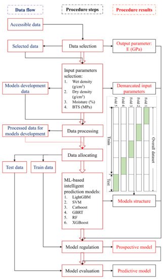
Figure 1. Systematic ML-based intelligent approach for predicting E.
2. Data Curation
In this research, 106 samples of soft sedimentary rocks, i.e., siltstone, claystone, and sandstone were collected from Block-IX of the Thar coalfield, as shown Figure 1, with the location map in the green. Then, the rock samples were prepared and partitioned according to the principles suggested by ISRM [45] and the ASTM [46] to maintain the same core size, and geological and geometric characteristics. In the laboratory of the Mining Engineering Department of Mehran University of Engineering and Technology (MUET), the experimental work was conducted on the studied rock samples to determine the physical and mechanical properties such as wet density (ρwet) in g/cm3, moisture (%), dry density (ρd) in g/cm3, Brazilian tensile strength (BTS) in (MPa), and elastic modulus (E) in (GPa). Figure 2 shows (a) collected core samples, (b) universal testing machine (UTM), (c) deformed core sample under compression for E test, and (d) deformed core sample for BTS test. The purpose of the UCS test was conducted on the standard core samples of NX size 54 mm in diameter with an applied load of 0.5 MPa/s using UTM according to the recommended ISRM standard to find the E of the rocks. Similarly, in order to find the tensile strength of the rock samples indirectly, we performed the Brazilian test using UTM. Figure 3 illustrates the statistical distribution of the input features and output in the original dataset used in this study. In Figure 3, the legend of boxplots can be explained as: ▭ 25~75%, ⌶ Range within 1.5 IQR, ─ Median line, and ○ Outliers.
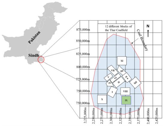
Figure 1. Location map of the study area.
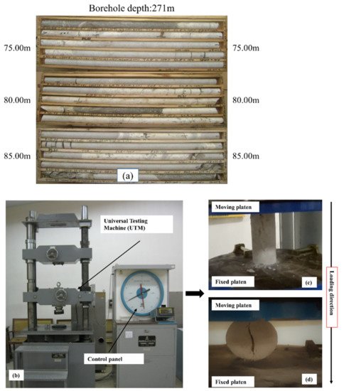
Figure 2. (a) Rock core samples for test, (b) uniaxial testing machine, (c) deformed rock core specimen under compression, and (d) deformed core sample for BTS test.
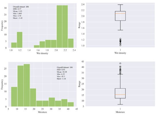
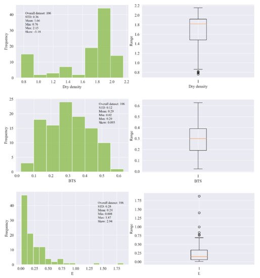
Figure 3. The statistical distribution of the input features and output in the original dataset.
In order to visualize the original dataset of E, the seaborn module in Python was employed in this study, and Figure 4 demonstrates the pairwise correlation matrix and distribution of different input features and output E. It can be seen that BTS is moderately correlated to the E, whereas ρwet and ρd are negatively correlated to the E. Moisture representation does not correlate with E. It is worth mentioning that each feature cannot be well correlated with E independently, so all features are evaluated together to predict E.
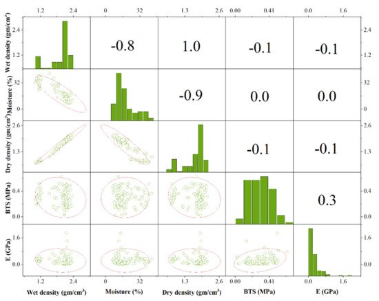
Figure 4. Pairwise correlation matrix and distribution of different input features and output E.
3. Developing ML-Based Intelligent Prediction Models
Light Gradient Boosting Machine
Light gradient boosting machine abbreviated as LightGBM, an open-source gradient boosting ML model from Microsoft, uses decision trees as the base training algorithm [47]. LightGBM puts continuous buckets of elemental values into separate bins with greater adeptness and a fast speed of training. It uses a histogram-based algorithm [48,49] to improve the learning phase, reduce consumption of memory, and integrate updated communication networks to enhance the regularity of training and is known as a parallel voting decision tree ML algorithm. The data for learning were partitioned into several trees, and local voting techniques were executed in each iteration to select top-k elements and gain globing voting techniques. As shown in Figure 5, LightGBM operates the leaf-wise approach to identify the leaf with the maximum splitter gain. LightGBM is best adopted for regression, classification, sorting, and several ML schemes. It builds a more complex tree than the level-wise distribution method through the leaf-wise distribution method, which can be considered as the main component of the execution algorithm with greater effectiveness. For all that, it can cause overfitting; however, by using the maximum depth element in LightGBM, it can be disabled.
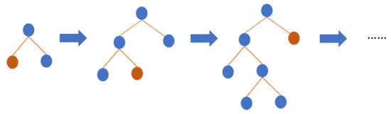
Figure 5. The general structure of LightGBM.
LightGBM [47] is a widespread library for performing gradient boosting, with some modifications intended. The implementation of gradient boosting is mainly focused on algorithms for building a computational system. The library includes tenfold training hyperparameters to validate the implementation of the framework in different scenarios. The implementation of LightGBM also demonstrates advanced capabilities on CPUs and GPUs, which can work like gradient boosting with multifold integrations, comprising column randomization, bootstrap subsampling, and so on. The main features of LightGBM are gradient-based one-sided sampling and unique attribute bundling. Gradient-based one-sided sampling is a sub-sampling technique used to construct the base tree of learning data as an ensemble. In the AdaBoost ML algorithm, the purpose of this technique is to increase the significance of samples with greater likelihood that are connected with samples with higher gradients. When gradient-based one-sided sampling is executed, the base learner’s learning data are articulated based on the top portion of samples with greater gradients (a) plus the portion of arbitrary orders (b) recouped from samples with lower gradients. To compensate for changes in measurement propagation, samples from the lesser gradient class are organized together and weighted by (1 − x)/y, and at the same time, computing the data gain. In contrast, the unique attribute bundling technique accrues meager elements into an individual element. This can be ended in the absence of impeding any information when these elements do not contain a non-zero number of coincidences. Both mechanisms predict a gain in the complementary learning rate.
This entry is adapted from the peer-reviewed paper 10.3390/su14063689
This entry is offline, you can click here to edit this entry!