Your browser does not fully support modern features. Please upgrade for a smoother experience.
Please note this is an old version of this entry, which may differ significantly from the current revision.
Subjects:
Engineering, Mechanical
Substantial gains and savings of resources of time and money can be gained through the use of modelling and simulation to understand material system performance. Since for development of the new materials validation is expensive and time-consuming, the bottleneck is time and funding—modelling might be the way to replace testing programs, which would be beneficial for providing new innovative materials faster to the market.
- modelling
- lifetime prediction
- accelerated testing methods
- durability
- mechanical properties
- creep
- fatigue
1. Arrhenius Model
The Arrhenius model is widely used when temperature is the dominant accelerating factor in ageing. It is assumed that a single dominant degradation mechanism does not change during the exposure period, while the degradation rate is accelerated with an increase of exposure temperature [14]. The Arrhenius relation is given by
where K is a reaction rate or degradation rate, A is a constant related to material and degradation process, Ea is the process activation energy, R is the universal gas constant, and T is the absolute temperature. The degradation rate is proportional to the inverse time for degradation of a mechanical property for a given value set by the lifetime criterion, and log(t) vs. 1/T is a linear function with the slope Ea/R (Figure 1). The Arrhenius relationship is widely used for lifetime predictions of polymers and composites through monitoring ultimate mechanical properties and their retention, e.g., tensile strength, interfacial shear strength, creep strength, and fatigue strength [6,21].
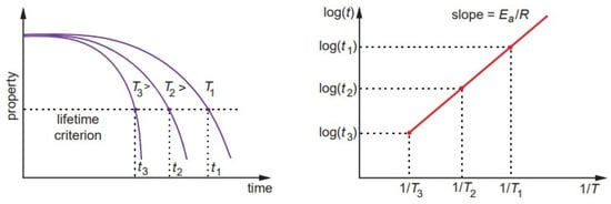
Figure 1. Lifetime prediction according to the Arrhenius model.
The durability prediction methodology in most studies is based on the time shift concept [8,21,22,23,24,25,26,27]. According to Equation (1), the time shift factor (TSF) for two different exposure temperatures T1 and (T1< T2) can be calculated as
Equation (2) has been further used in the predictive methods based on superposition principles and assessment of the temperature shift factors. The activation energy in Equations (1) and (2) is commonly evaluated by thermal analysis methods, e.g., differential scanning calorimetry or thermogravimetric analysis by measuring heat capacity changes or mass losses under different heating rates. Alternatively, Ea can be determined by dynamic thermal mechanical analysis (DMTA) assessing Tg dependence on the test frequency [28,29].
Some recent studies considering the Arrhenius model and TSF approach for predicting the long-term strength of various FRP are listed in Table 1. Note that this methodology can be applied for assessment of tensile strength [22,30], interlaminar shear strength [23,26,27] or bond strength [25], under both static and fatigue loadings [26]. The accelerating temperature effect can also be coupled with other factors, e.g., absorbed water. For instance, Gagani et al. [26] applied the time shift concept to assess interlaminar shear fatigue lifetime of GFRP considering the effects of temperature and water immersion. The glass transition temperature of the material, and its decrease due to absorbed water, was used in Equation (2), enabling representation of both dry and water saturated samples in the same Arrhenius-based master curve.
Table 1. A condensed list of recent works on methods for predicting long-term mechanical properties of polymers and polymer composites.
| Prediction Method | Material | Property | Ref. |
|---|---|---|---|
| Rate models | |||
| Arrhenius model | GFRP | Tensile strength | [22,30] |
| GFRP | ILSS | [27] | |
| GFRP | Fatigue ILSS | [26] | |
| GFRP bars | Tensile strength | [8] | |
| CFRP/GFRP rods | ILSS | [23] | |
| BFRP bars | Residual tensile strength | [24] | |
| GFRP rods | Bond strength | [25] | |
| Eyring’s model | PA6,6, PC, CFRP | Creep failure time | [31] |
| Zhurkov’ model | PP | Fatigue strength | [32] |
| Superposition principles | |||
| Time–temperature (TTSP) | Epoxy | Creep compliance | [28,33] |
| Epoxy | Stress relaxation | [34] | |
| Filled epoxy | Stiffness/Relaxation modulus | [35] | |
| PMMA | Creep compliance | [36] | |
| Polyvinyl chloride, epoxy | Stress threshold of LVE | [37,38] | |
| Flax/vinylester | Creep compliance | [39] | |
| CFRP | Creep compliance | [40,41] | |
| CFRP, GFRP | Static/creep/fatigue strength | [42,43] | |
| Time–moisture (TMSP) | Epoxy | Creep compliance | [28,33] |
| Epoxy | Relaxation/storage modulus | [44,45,46,47,48] | |
| Epoxy-based compounds | Relaxation modulus | [49] | |
| Vinylester | Creep strain | [50] | |
| Polyester | Creep strain | [51] | |
| PA6, PA6,6 | Storage modulus | [47,52] | |
| CFRP, GFRP | Fatigue strength | [53] | |
| Time–stress (TSSP) | PA6 | Creep strain | [54] |
| PMMA | Creep compliance | [36,55,56] | |
| HDPE | Creep strain/lifetime | [57] | |
| Polycarbonate | Creep compliance | [58] | |
| PA6,6 fibres | Creep strain | [59] | |
| Glass/PA, PP, HDPE | Creep compliance | [60] | |
| HDPE/wood flour | Creep strain | [61] | |
| Graphite/epoxy FRP | Creep strain | [62] | |
| Kevlar yarns, PA6, epoxy | Creep strain (stepped isostress test) | [63,64,65] | |
| Coupled | |||
| TTSP + TMSP | Epoxy | Creep compliance | [28] |
| TTSP + TMSP | PA6,6 | Storage modulus | [52] |
| TTSP + TMSP | Acrylate-based polymers | Storage modulus | [66] |
| TTSP + TMSP | CFRP, GFRP | Static/creep/fatigue strength | [53,67] |
| TTSP + TSSP | HDPE/wood flour | Creep strain | [61] |
| TASP+TMSP | Epoxy, polyester | Creep compliance, stress relaxation | [44,45] |
| TTSP+TASP | Epoxy | Relaxation modulus | [34,68] |
| TTSP+TASP+TSSP | PMMA | Creep strain | [55] |
| Plasticity-controlled failure | PP, PP/CNT, glass/PP, carbon/PEEK, PC/GF, PA6 | Lifetime (tensile, creep, fatigue) | [69,70,71,72,73,74] |
| PA6,6, PC, CFRP | Creep lifetime | [31] | |
| Parametric methods | HDPE | Creep lifetime (Larson–Miller, Monkman–Grant) | [57] |
| GFRP | Creep lifetime (Monkman–Grant) | [75] | |
| Rubber-bonded composite | Creep lifetime (Larson–Miller) | [76] | |
| Adhesive anchor in concrete | Creep lifetime (Monkman–Grant) | [77] | |
| Short fibre thermoplastics | Fatigue lifetime (Larson–Miller) | [78,79] |
2. Eyring’s Model
The reaction rate of a process can rely on several stressors. For example, nonthermal stresses such as humidity, voltage and mechanical stress may also play a significant role in accelerating degradation [14]. The Eyring model is based on chemical reaction-rate theory and describes how the rate of degradation of a material varies with stress. It is assumed that the contribution of each stressor to the reaction rate is independent; thus, one could multiply the respective stress contributions to the rate of reaction. The model is closely related to the Arrhenius model and is based on the fact that the logarithm of the reaction rate is inversely proportional to absolute temperature (Equation (1)).
According to Eyring’s thermal activation flow theory, the strain rate (or the characteristic time) is given by the relationship
3. Zhurkov’s Model
Zhurkov developed the kinetic theory of strength of solids using temperature and tensile stress [32,81]. The relationship for calculation of the fracture lifetime tf is similar to Equation (3), while the coefficient γ referred to as the lethargy coefficient is linked to lattice structure and defects in it. In the general case of nonisothermal tests and σ varying in time (e.g., creep and fatigue tests), the fracture probability with account of the linear damage accumulation concept is given by the following equation [32,75,82]:
where t0 is the time constant.
Zhurkov’s model initially developed for metals often could not give accurate lifetime predictions for polymers owing to the sensitiveness of their mechanical properties to strain rate and uncertain distinctions between the elastic and plastic ranges. As a result, the parameters involved in Equation (4) are interrelated stress, temperature, and strain-rate dependent functions. The kinetic concept of strength is applied to model fatigue damage evolution [32,83]. Hur et al. developed a modified Zhurkov’s fatigue life model introducing strain-rate-dependent lethargy coefficient and applied it to polypropylene reinforced with glass fibres [32]. The stress-based failure cycles in the ranges of low- and high-cycle fatigue were predicted and successfully validated by the proposed modified strain-rate model. The kinetic strength model applied to lifetime predictions of biodegradable polymers is discussed in the review paper by Laycock et al. [5]. For this type of material, Zhurkov’s equation is coupled with broader biodegradation models enabling assessment of stress effects on the lifetime via lowering the activation energy for chain scission.
This entry is adapted from the peer-reviewed paper 10.3390/polym14050907
This entry is offline, you can click here to edit this entry!