The Global Navigation Satellite System (GNSS) plays a pivotal role in our modern positioning, navigation and timing (PNT) technologies. GNSS satellites fly at altitudes of approximately 20,000 km or higher. This altitude is above an ionized layer of the Earth’s upper atmosphere, the so called “ionosphere”. Before reaching a typical GNSS receiver on the ground, GNSS satellite signals penetrate through the Earth’s ionosphere. The ionosphere is a plasma medium consisting of free charged particles that can slow down, attenuate, refract, or scatter the GNSS signals. Ionospheric density structures (also known as irregularities) can cause GNSS signal scintillations (phase and intensity fluctuations). These ionospheric impacts on GNSS signals can be utilized to observe and study physical processes in the ionosphere and is referred to ionospheric remote sensing. This entry introduces some fundamentals of ionospheric remote sensing using GNSS.
- GNSS
- ionosphere
- remote sensing
1. GNSS Introduction
The positioning, navigation, and timing (PNT) provided by the Global Navigation Satellite System (GNSS) forms a ubiquitous technological infrastructure in modern society. The high-level GNSS positioning is simply based on the principle of trilateration. To determine the unknown location (x, y, z) of a GNSS receiver as shown in Figure 1, for simplicity let us assume the locations of three beacon GNSS satellites in the sky are known beforehand (transmitted by the GNSS satellites to the receiver via navigation messages). When the receiver acquires and tracks the incoming GNSS signals from the three satellites, it can determine the signal propagation time Δt (transmission time minus reception time). Assume the GNSS signals propagate at the speed of light (c), the distances from the receiver to the 3 beacon satellites (R1, R2, and R3) can be estimated by multiplying c with Dt. Then, a set of trilateration equations can be established as:

Given xm, ym, zm, Δtm, and c are known, the three unknowns x, y, and z can be determined by solving the three equations simultaneously and the solutions will give two positions (one outside of the Earth, one on the surface on the Earth). It is important to note in reality, there is an unknown bias in the signal propagation time from every beacon satellite due to a common time error from the inaccurate receiver clock (δt). Therefore, an additional clock bias term must be introduced as the fourth unknown, implying in reality that four satellites are needed to determine the receiver position. Consequently, an additional GNSS beacon satellite needs to be tracked to obtain a fourth sphere equation.

This set of four equations, involving reception of at least four GNSS satellite signals, forms the underlying algorithm to solve a simple static positioning problem in the 3D space including the receiver clock bias.
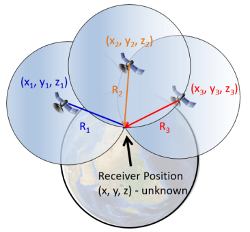
Figure 1. Trilateration principle of GNSS positioning.
By definition, GNSS are satellite navigation systems with global signal coverage. Currently, there are four operational GNSS constellations: USA’s Global Positioning System (GPS), Russia’s Global’naya Navigatsionnaya Sputnikovaya Sistema (GLONASS), European Union’s Galileo, and China’s BeiDou Navigation Satellite System (BDS, formerly known as COMPASS). As of October 2021, the GPS, GLONASS, and Beidou constellations are fully operational. The Galileo constellation is expected to reach a full operational capability (FOC) stage soon. A brief status summary of four GNSS constellations is given in Table 1.
Table 1. Current status of GNSS constellations (* n stands for GLONASS frequency channel number)
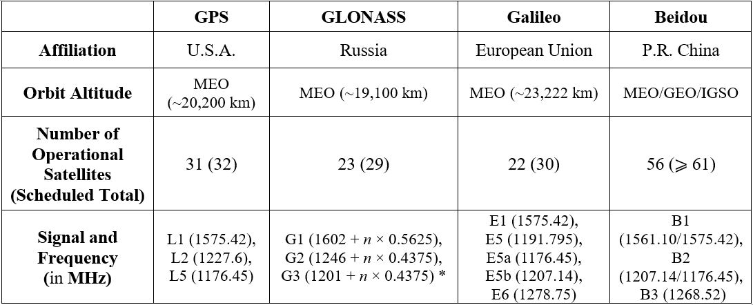 The GPS satellites are located within six different orbital planes of medium Earth orbit(MEO) with an altitude of ∼ 20,200 km. Each two neighboring orbital planes are separated by 60 degrees in Ω (longitude of the ascending node). The inclination angle of all GPS satellites is approximately 55 degrees. The orbital period of all GPS satellites is approximately 12 h. By design, a GPS receiver at any place on the Earth’s open surface should be able to track at least six line-of-sight (LOS) direction satellites. The GPS constellation is designed with a total number of 32 satellites in orbit. Currently among the 31 operational GPS satellites, 11 satellites broadcast the L1 (1575.42 MHz) signal only, 7 satellites broadcast the L1 and L2 (1227.6 MHz) signals, and 13 satellites broadcast the L1, L2 and L5 (1176.45 MHz) signals. The transmission of these GPS civilian radio-frequency (RF) signals is based on the Code Division Multiple Access (CDMA) spread-spectrum technology. The details of GPS signal structure can be found in the Interface Control Documents (ICD) [1]. The latest status of the GPS constellation can be found at the U.S. Coast Guard Navigation Center website [2].
Currently, 24 operational GLONASS satellites are located within three different MEO orbital planes with an altitude of ∼19,100 km, which indicates GLONASS satellites’ orbital period is ∼11 h 15 min. Each two neighboring GLONASS orbital planes are separated by an Ω of 120 degrees, and all satellite inclination angles are approximately 64.8 degrees. In contrast to the GPS constellation, the transmission of GLONASS civilian RF signals is based on the frequency division multiple access (FDMA) technique. Therefore, the RF transmitting frequencies under the same frequency band on different GLONASS satellites are different. 22 out of the 24 GLONASS satellites transmit dual frequency bands, where their G1 center frequency is 1602 + n × 0.5625 MHz and G2 center frequency is 1246 + n × 0.4375 MHz (where n is the satellite frequency channel number). The other two GLONASS satellites transmit an additional frequency band, G3, with a center frequency of 1201 + n × 0.4375 MHz. The details of GLONASS signal structure can be found in their ICDs [3]. The latest status of the GLONASS constellation can be found at the Russian Information and Analysis Center for Positioning, Navigation and Timing website [4].
Currently, 22 operational Galileo satellites are located within three different MEO orbital planes with an altitude of ∼23,200 km, which gives an orbital period ∼14 h 7 min for the Galileo satellites. The FOC stage of Galileo is expected to be composed of 30 satellites in total. Each neighboring Galileo orbital plane is separated by an Ω of 120 degrees, and all satellite inclination angles are approximately 56 degrees. The Galileo constellation utilizes
the CDMA technique for RF signal transmission. All the Galileo satellites broadcast E1 (1575.42 MHz), E5a (1176.45 MHz), E5b (1207.14 MHz) and E6 (1278.75 MHz) civilian signals. Galileo receivers may receive the E5 AltBOC modulation signal, a modified version
of a Binary Offset Carrier (BOC) with a center frequecy of 1191.795 MHz. The details of Galileo signal structure can be found in their ICDs [5]. The latest status of the Galileo can
be found at the European GNSS Service Centre website [6].
The orbits of the Beidou constellation are more complicated than the other three constellations. Out of the 43 currently operational Beidou satellites, 5 satellites are in the geostationary orbit (GEO) over the Asian sector; 10 satellites are in inclined geosynchronous orbits (IGSO) with an altitude of ∼35,786 km and an inclination angle of 55°; 28 satellites are in MEO with a nominal altitude of ∼21,528 km. The MEO satellites are separated within three orbital planes (equally divided by 120 degrees) with an orbital period of ∼12 h and 53 min. Compared to other GNSS constellations, the more complicated orbit geometry of the BDS can increase positioning accuracy by providing lower horizontal, vertical and temporal dilution of precision (DOP) particularly in a large portion of the eastern hemisphere region (60° S–60° N and 50° E–170° E) [7]. More BDS satellites will be launched to complete the full constellation with at least 49 satellites in total. Beidou second generation satellites transmit public RF signals in three different frequency bands: B1 (1561.098 MHz), B2 (1207.14 MHz) and B3 (1268.52 MHz). Beidou third generation satellites also transmit three different frequency bands of public signals: B1 (1575.42 MHz), B2 (1176.45 MHz) and B3 (1268.52 MHz). The details of BDS signal structure can be found in their ICDs [8]. The latest status of the Beidou constellation can be found at the Test and Assessment Research Center of China Satellite Navigation Office website [9].
2. GNSS Observables and Ranging Errors
In order to achieve PNT, a standard GNSS receiver’s measurement module must generate GNSS observables and the receiver’s positioning module must properly model each ranging error for GNSS observables. GNSS observables refer to the basic measurements produced from a GNSS receiver, including pseudorange, carrier-phase, and Doppler shift. Together with the epoch time and the carrier-to-noise density ratio (often denoted as C/N0), these data are conventionally stored in a observation file based on the receiver independent exchange format (RINEX) [10].
Pseudorange (also known as code-range) refers to the sum of the real range and the range equivalent of various ranging errors or offsets. Pseudorange (P) can be defined as:

where m denotes a specific GNSS satellite number. R is the true geometric range from the
satellite to receiver’s antenna phase center in meters, c is the speed of light in vacuum in meters per second, δT is the satellite clock bias in seconds, δt is the receiver clock bias in seconds, I is the ionospheric signal delay in meters, T is the troposphere signal delay in
meters, M is the multipath effect delay in meters, D is the error caused by the geometric
dilution effect in meters, W refers to all other noise effects (e.g., receiver noise, relativity
effects). The standard unit of P is meters.
Doppler shift (fD or simply Doppler) is the frequency shift caused by the relative motion between a GNSS satellite (transmitter) and receiver (antenna). fD is related to the satellite radial velocity (vr), which is equal to the pseudorange rate:
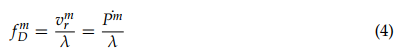
where λ is the wavelength of the GNSS signal being used. fD is typically not used tocompute navigation solutions, but instead used to determine the receiver velocity. The standard unit of fD is Hz.
Carrier-phase (or beat carrier-phase) refers to the time integral of the carrier Doppler shift. Carrier-phase (CP) can be defined as:

where N is the carrier-phase measurement ambiguity (sometimes known as integer ambiguity). CP typically is measured in number of cycles of the carrier signals being received and tracked. The relationship between fD and CP can be expressed as:
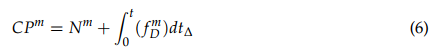
where t∆ is the elapsed time during a carrier-phase measurement.
3. Ionospheric Characteristics and Phenomena
The ionosphere is an ionized layer of the Earth’s upper atmosphere. Due to the solar radiation, the neutral particles in the Earth’s atmosphere are converted to electrons and ions. Overall, these electrons are concentrated in the altitude range from ∼60 km to 1000 km but their characteristics are spatially and temporally dynamic [11]. In equatorial and low-latitude regions (latitude < 30 degrees North/South), the magnetic field is nearly horizontal and ionospheric electron density is typically higher than other regions due to the high solar angle effect. Equatorial Spread F (ESF) or Equatorial plasma bubbles (EPB) form density structures in the ionosphere and have a typical scale size between 1° (∼115 km) and 4° (∼460 km) [12]. Additionally, plasma irregularities driven by plasma instabilities can be detected to smaller scale (∼10-1 to 103 m) as well. The high-latitude (or polar) ionosphere is the region above 60° magnetic latitude (e.g., auroral zone, polar cap), where plasma instabilities and other dynamic processes (e.g., coupling physics between the magnetosphere, ionosphere and thermosphere) cause ionospheric structures and irregularities [11]. Under the influence of the nearly vertical geomagnetic field as well as the horizontal variation of plasma density and electric fields driven by plasma instabilities, various multi-scale (∼10-2 to 105 m) ionospheric structures lead to phenomena such as aurora (and the associated arcs), sub-auroral polarization streams (SAPS), as well as polar tongues of ionization (TOI). A broad range of observation techniques must be used to study these multi-scale space weather phenomena which span seven orders of magnitude or more in space and time scales.
Aurora, one of the most famous and important space weather phenomena, is typically seen as a visual phenomenon caused by charged particle precipitation along polar geomagnetic field lines and subsequent interaction with the neutral particles in the upper
atmosphere. The energetic charged particles are often driven by the solar wind [11]. The length of auroral arcs can range from 100 to 1000 km, the width can range from 50 m to 10 km, and the altitude (maximum energy of particles in the primary beam) is typically from 80m to 400 km [13]. SAPS often refers to a sunward plasma drift/convection in the sub-auroral region with an approximate spatial span of ∼3°–5° latitudinally and temporal duration of several hours in the evening sector [14]. TOI is a continuous stream of cold plasma enhancement with an entrainment pattern of high-latitude convection. The spatial
scale of TOI can range from about 100 to 1000 km [15]. A hardware-in-the-loop simulation of TOI and its impact on GNSS was reported by [16].
4. Ionospheric Remote Sensing
GNSS is not only the ubiquitous modern technology for PNT, but also a versatile remote sensing tool for many areas (e.g., space weather, geodesy, geophysics, and oceanography). For example, GNSS is widely applied to ionospheric remote sensing. Plasma physics describes the basic science of the ionosphere. An important parameter—plasma frequency (ωP) can be defined as:
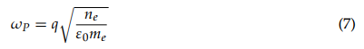
where q is elementary charge (≈1.6 × 10⁻¹⁹ C); ne is electron density; ε0 is the permittivity of free space; and m e is the electron rest mass. For radio waves with frequencies below ωP, typically 10’s of MHz, the ionosphere can reflect the RF waves (e.g., amplitude modulated radios) and enables long distance over the horizon radio communications globally.
For radio waves frequencies above ωP, such as GNSS, the signals penetrate through the ionosphere. Due to the difference in index of refraction in the ionosphere compared to a vacuum (free space), the ionosphere can delay, attenuate, disturb or induce Faraday rotation on GNSS signal propagation. The index of refraction depends on electron density
and RF wave frequency [17]. These ionospheric effects can dramatically degrade the PNT accuracy, precision, and integrity of GNSS. Conversely, GNSS can be (and has been) utilized to monitor and study the ionosphere.
Associated with the ionospheric delay effect, the total electron content (TEC) of the ionosphere can be measured by multi-frequency GNSS receivers on the ground or in space.
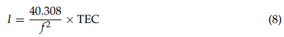
TEC is defined as the total number of electrons within a cross-sectional volume along the LOS between two points (e.g., a GNSS satellite and a ground-based GNSS receiver): TEC = R0R nedr, where R is the LOS’s distance. The TEC is measured in units of number of electrons per m2, but more often expressed in units of TECU (1016 electrons/m2). The ionospheric delay I (measured in meters) on a ranging Equation (Equations (4) and (6)) with a specific frequency band can be expressed in terms of TEC as [17]:
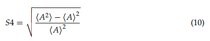
where f is the GNSS signal frequency. Using the pseudorange from two GNSS different frequency bands (e.g., GPS L1 and L2), the TEC can be measured based on the following formula:
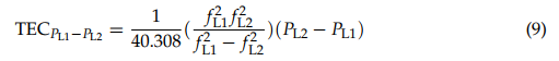
where fL1 is GPS L1 frequency, fL2 is GPS L2 frequency, PL1 is GPS L1 pseudorange, and PL2 is GPS L2 pseudorange. Due to the differential code bias (DCB), an offset caused by different hardware delays on GNSS code/pseudorange observations with different signal frequencies, an additional DCB bias term needs to be accounted for when implementing Equation (10). More details about DCB estimations can be found at [18]. The MIT Madrigal database gathers thousands of multi-frequency GPS/GNSS receiver data to create global TEC maps [19] as shown in Figure 2, which is advantageous for global ionospheric weather monitoring and studies. Note, vertical TEC (VTEC) is an integration of the electron density along the direction perpendicular to the ground standing. There are several other global TEC monitoring systems/institutes, such as NASA Jet Propulsion Laboratory (JPL) [20], International GNSS Service (IGS) [21], and United States’ National Oceanic and Atmospheric Administration (NOAA) [22].
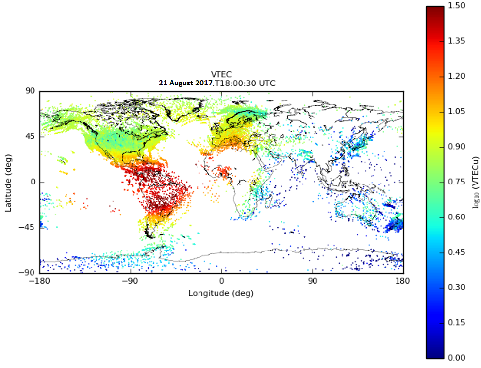 Figure 2. A global VTEC map from MIT Madrigal world-wide GPS receiver network [23].
Other than ionospheric delay, ionospheric irregularities can cause GNSS scintillations (rapid fluctuations in signal’s intensity or/and phase). According to [24], ionospheric irregularities are “small-scale structures in the ionospheric plasma density generally oriented so that the plasma density variations occur rapidly across the geomagnetic field but slowly (or not at all) along the geomagnetic field”. Two ionospheric scintillation indices are used to quantify the scintillation severity:
(a) S4 (amplitude scintillation index): the ratio of the standard deviation of the signal power to the average signal power computed over a period of time (typically 1 min) as defined by [25]:
where A is the signal intensity or power, and ⟨⟩ denotes ensemble averaging (≈time averaging).
(b) sigma phi or σϕ (phase scintillation index): the standard deviation of σ in radians, where σ is the refractive component of the GNSS signal phase as defined by [25] and ϕdetr is the detrended phase.  Ionospheric irregularities may simultaneously lead to GNSS ranging errors (TEC delay) and GNSS signal phase scintillations. The relationship between the GPS phase scintillations and TEC variation can be expressed as (described in detail in [26]):
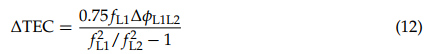
where the differential carrier phase between L1 and L2 frequency bands (∆ϕL1L2) is proportional to TEC variation (∆TEC).
As shown in Figure 3, an example GPS scintillation event observed at the Antarctic McMurdo scintillation Station from MIT Madrigal contains both high amplitude and phase scintillation measurements. The background color represents VTEC level in a similar way in Figure 2, and the red circles represent S4 in Figure 3a and sigma phi (σϕ) in Figure 3b. On 7 January 2014, the polar ionospheric irregularities and density structures in the southern polar region induced by an incoming solar storm caused an observation of this scintillation event (with relatively high S4 and σϕ) using ground-based GPS receivers.
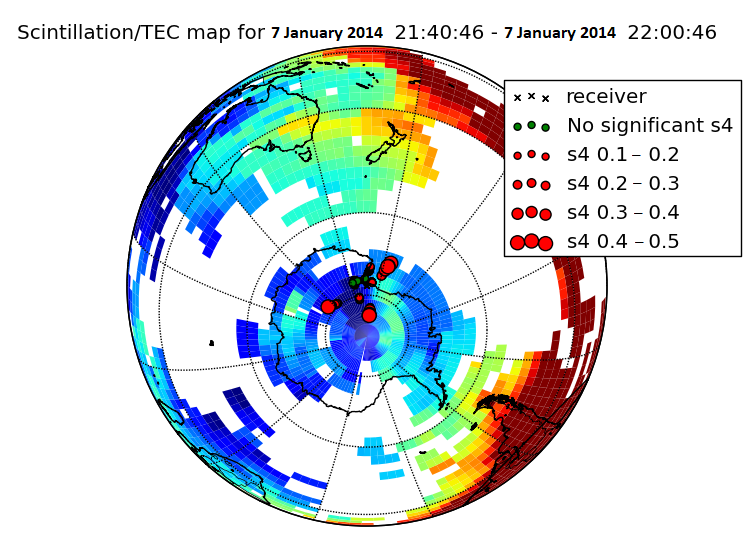
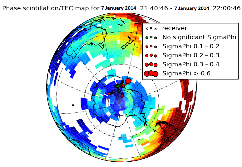 Figure 3. An example GPS scintillation event observed at the Antarctic McMurdo scintillation Station from MIT Madrigal. Adapted from [27] (a) S4 measurement; (b) SigmaPhi (σϕ) measurement.
GNSS is widely used to measure S4 and σϕ in order to observe and study the associated ionospheric irregularities. GNSS phase scintillations can cause cycle slips in carrier-phase and put pressure on the tracking loops of GNSS receivers. Severe GNSS scintillations can even lead to GNSS receiver loss-of-track and thus reduce positioning accuracy and availability. A great number of ground-based receivers are deployed in different regions around the world to detect and measure ionospheric space weather including the plasma irregularities that disturb GNSS signals. For instance, the chain of autonomous adaptive low-power instrument platforms (AAL-PIP) [28] on the East Antarctic Plateau has been used to observe ionospheric activity in the South Polar region. Together with six groundbased magnetometers, four dual frequency GPS receivers of the AAL-PIP project have been used to capture ionospheric irregularities and ultra-low frequency (ULF) waves associated with geomagnetic storms by analyzing the GPS TEC and scintillation data collected in Antarctica [29]. Furthermore, the ESA Space Weather Service Network is hosting several ionospheric scintillation monitoring systems developed by the German Aerospace Center (DLR), Norwegian Mapping Authority (NMA), and Collecte Localisation Satellites (CLS) [30]. Figure 4 gives a high-level illustration of two ionospheric impacts on GNSS—ranging errors and scintillation.
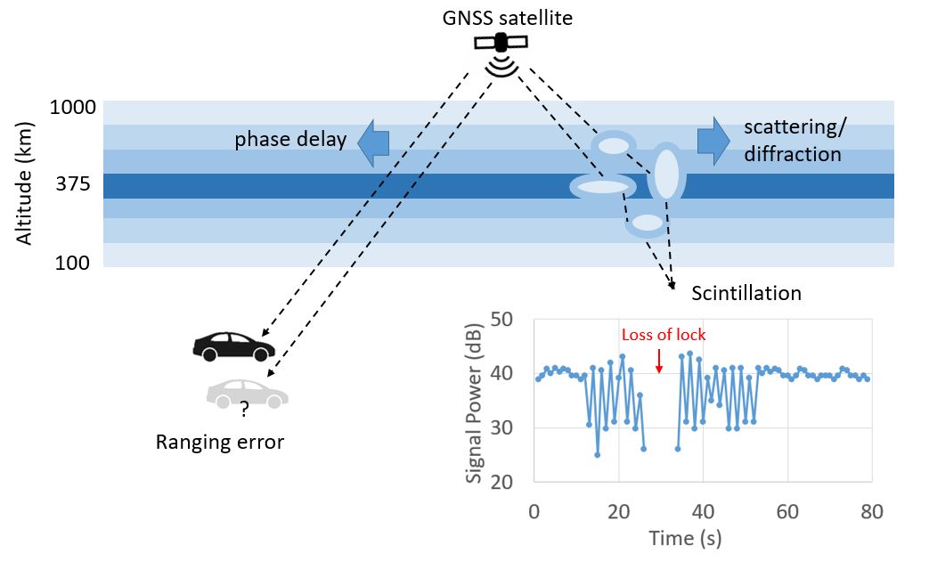 Figure 4. An illustration of ionospheric impacts on GNSS.
Besides ground-based GNSS ionospheric remote sensing, there are space-based approaches that utilize the spaceborne GNSS receivers on satellites for ionospheric radio soundings. For example, the Constellation Observing System for Meteorology, Ionosphere, and Climate (COSMIC) mission uses the radio occultation technique (a bending effect on the GNSS signals propagating through the Earth’s upper atmosphere) to measure space-based TEC and scintillations, detect ionospheric irregularities, and reconstruct global electron density profiles using ionospheric tomography techniques [31]. Using low-Earth-orbit GNSS receivers sensors in proximity together with spacecraft formation flying techniques, the ionospheric TEC, electron density, and scintillation index can also be measured globally with high flexibility [32–34].
5. Conclusions and Prospects
Fundamental physics and engineering of GNSS and ionospheric remote sensing are
introduced in this entry. It is important to monitor and understand the ionospheric impact on GNSS, because the ionosphere can cause delays or scintillation of GNSS signals which eventually degrade the PNT solutions from GNSS. As a reflection of ionospheric ionization level, TEC is an integration of the electron density along the LOS between two points. The larger the TEC, the larger ranging offset in the GNSS observable caused by the ionosphere.
S4 and σϕ are the two commonly used ionospheric scintillation indexes to quantify the GNSS signal fluctuation level in the amplitude and phase domain, respectively. Ionospheric irregularities can cause scintillations of GNSS signals, which may lead to signal attenuation, carrier phase cycle slip or even loss of lock. The ubiquitous GNSS is a powerful engineering tool for ionospheric remote sensing. Ionospheric remote sensing studies using groundbased GNSS receivers have been conduced over the past several decades, while ionospheric measurement using space-based GNSS techniques is emerging rapidly and providing much higher coverage and flexibility.
Author Contributions: Conceptualization, Y.P. and W.A.S.; methodology, Y.P.; software, Y.P.; validation, Y.P. and W.A.S.; formal analysis, Y.P.; investigation, Y.P.; resources, Y.P. and W.A.S.; writing—original draft preparation, Y.P.; writing—review and editing, W.A.S.; visualization, Y.P.; supervision, W.A.S. All authors have read and agreed to the published version of the manuscript.
Funding: This work is supported by the AFOSR (Grant No. 13-0658-09) and Virginia Tech.
Data Availability Statement: GPS TEC data products and access through the Madrigal distributed data system are provided to the community by the Massachusetts Institute of Technology under support from US National Science Foundation grant AGS-1952737. Data for the TEC processing is provided from the following organizations: UNAVCO, Scripps Orbit and Permanent Array Center, Institut Geographique National, France, International GNSS Service, The Crustal Dynamics Data Information System (CDDIS), National Geodetic Survey, Instituto Brasileiro de Geografia e Estatística, RAMSAC CORS of Instituto Geográfico Nacional de la República Argentina, Arecibo Observatory, Low-Latitude Ionospheric Sensor Network (LISN), Topcon Positioning Systems, Inc., Canadian High Arctic Ionospheric Network, Institute of Geology and Geophysics, Chinese Academy of Sciences, China Meteorology Administration, Centro di Ricerche Sismologiche, Système d’Observation du Niveau des Eaux Littorales (SONEL), RENAG : REseau NAtional GPS permanent, GeoNet—the official source of geological hazard information for New Zealand, GNSS Reference Networks, Finnish Meteorological Institute, SWEPOS—Sweden, Hartebeesthoek Radio Astronomy Observatory, TrigNet Web Application, South Africa, Australian Space Weather Services, RETE INTEGRATA NAZIONALE GPS, Estonian Land Board, Virginia Tech Center for Space Science and Engineering Research, and Korea Astronomy and Space Science Institute.
Acknowledgments: The authors would like to thank Anthea Coster, Greg Earle, Michael Ruohoniemi, Robert Clauer, and Jonathan Black for their comments and inputs on our work.
Conflicts of Interest: The authors declare no conflict of interest.
Abbreviations
The following abbreviations are used in this manuscript:
| GNSS PNT GPS GLONASS BDS |
Global navigation satellite system Positioning, Navigation and Timing Global Positioning System Global’naya Navigatsionnaya Sputnikovaya Sistema BeiDou Navigation Satellite System |
| FOC MEO LOS RF CDMA |
Full Operational Capability medium Earth orbit line-of-sight radio-frequency Code Division Multiple Access |
| FDMA | Frequency Division Multiple Access |
| BOC GEO IGSO DOP RINEX |
Binary Offset Carrier geostationary orbit inclined geosynchronous orbits dilution of precision Receiver Independent Exchange Format |
| P CP ESF |
Pseudorange Carrier-phase Equatorial Spread F |
| EPB SAPS TOI TEC DCB MIT AAL-PIP ULF COSMIC |
Equatorial plasma bubbles sub-auroral polarization streams tongues of ionization total electron content differential code bias Massachusetts Institute of Technology Autonomous Adaptive Low-Power Instrument Platforms ultra-low frequency Constellation Observing System for Meteorology, Ionosphere,and Climate |