1. Introduction
Hot-melt extrusion (HME) is a rapidly growing technology in the pharmaceutical industry, for the preparation of various dosage forms, including granules, pellets, tablets, and implants. The HME process offers many advantages relative to other pharmaceutical processes, one of the major benefits being that HME can enhance the bioavailability and solubility of poorly soluble drugs. Further, as a solvent-free process, it is free of harsh environmental toxicants and no additional step for solvent recovery is required, unlike solvent evaporation and spray drying. HME is also relatively easy to scale-up, and it is a continuous process [
1].
As with all pharmaceutical products, polymer–drug extrudates that are produced using HME must undergo rigorous quality analysis and typically undergo thermal, rheological, mechanical, and chemical characterisation. For thermal analysis, DSC and TGA are widely used to measure the percentage of crystallinity, the glass transition temperature (T
g), and the change in weight. The results of these methods have been used to predict the miscibility, solid state, and stability of the polymer–drug matrix [
2,
3,
4,
5,
6,
7,
8,
9,
10,
11,
12,
13,
14,
15,
16,
17,
18,
19]. Rheological analysis is used to provide information about the behaviour of the polymer–drug system under the high temperature and stresses experienced in the process itself [
20,
21,
22,
23]. HPLC is used to monitor the drug/additive content in the extrudate [
4,
5,
14,
18,
19]. FT-IR, Raman, and NIR have been employed post-production to study the stability and for analysing the drug content in the polymer–drug matrix [
2,
4,
10,
18,
19,
24]. Physicomechanical testing [
25,
26] and dissolution testing [
27,
28] are also performed for product quality assurance. The main disadvantage of these off-line, lab-based methods is that there is a long lag between processing and feedback on product quality, which makes process control very challenging. HME is a continuous process, but the long testing time for product quality assurance defeats this advantage of the process.
In 2004, the Food and Drug Administration (FDA) introduced the concept of using process analytical technology (PAT) [
29]. The main aim is to improve the understanding of the mechanism of the manufacturing process, enhance process monitoring, and to reduce the processing time. In the literature, spectroscopic techniques, including Raman [
2], NIR [
30], and UV–Vis spectroscopy [
31], have been widely implemented as PAT tools for in/on-line monitoring of the HME process, and an in-line slit die rheometer has also been implemented as a PAT tool in some studies [
32,
33]. Machine learning (ML) algorithms are generally used to infer the required information from in/on-line collected spectra.
A PAT tool, coupled with a machine learning algorithm, has been established as an effective way to monitor the HME process in real-time.
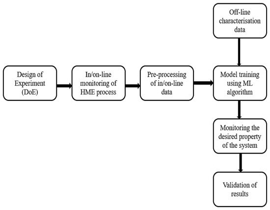
Figure 1 gives a schematic representation of the work flow for in/on-line monitoring of the HME process using PAT tools coupled with machine learning. Since 2004, many research studies have been reported, in which different machine learning algorithms have been applied to in-process data to analyse product and process parameters in real-time. The applications include the monitoring of product critical quality attributes (CQAs), including the following: the solid state of the polymer/drug [
2,
3]; API/additive concentration [
34,
35]; degradation of the polymer [
36,
37]; the particle size of additive/s [
31]; and mechanical properties [
33]. Other works have examined the monitoring of critical process properties (CPPs), including melt temperature [
38], pressure [
39], and viscosity [
40], and for process fault detection [
41].
Figure 1. Schematic representation of in/on-line monitoring of HME process with machine learning.
In recent years, many review papers have been published focusing on different aspects of the HME process [
1,
15,
42,
43,
44,
45,
46,
47,
48,
49,
50,
51,
52,
53,
54,
55,
56,
57,
58]. In this review, we focus specifically on the application of machine learning (ML) algorithms in the monitoring and control of the HME process. Greater process sensorization, coupled with algorithms for deriving intelligence from data, are key concepts of the Pharma 4.0 initiative for the digital transformation of the pharmaceutical industry, hence this review aims to establish the current state of the art of the HME process in this respect. We present and discuss the various data analytics and machine learning methods reported for the monitoring and control of HME, including the following: methods for the pre-processing of data, model training/calibration, the ability of the developed model to detect the effect of varying processing conditions, and the performance of models on unseen data. We summarise the contribution that machine learning has made to date in the monitoring and control of the HME process and discuss the main challenges and future potential of the field.
The remainder of the paper is organised as follows: First, a brief introduction is given to machine learning and the main data pre-processing techniques that are relevant to the HME process. The main body of the paper then reviews the applications of (i) PCA, (ii) PLS, and (iii) non-linear machine learning algorithms to the process, followed by the discussion and conclusions.
2. Machine Learning
Machine learning (ML) is generally defined as the ability of a computer to learn without being explicitly programmed. Machine learning algorithms train themselves to identify patterns in the data or make predictions based on past data, as opposed to modelling algorithms that are based on the prior physical/chemical knowledge of a system. A machine learning system can be predictive; descriptive (meaning that the system uses the data to explain what happened); or prescriptive (meaning that the system will use the data to make suggestions about what action to take). ML algorithms can be divided into the following three classes: supervised learning, unsupervised learning, and reinforcement learning [
59].
2.1. Supervised Machine Learning
In supervised learning, algorithms are provided with known/labelled input–output data [
59,
60]. In other words, supervised machine learning algorithms try to predict the results for an unknown output based on the patterns present in the labelled data set, i.e., the algorithm tries to approximate the mapping function from input to output variables. Regression and classification are categorised under supervised machine learning.
Classification algorithms classify training data into separate categorical classes/groups. All the samples of data in the training set are labelled. The purpose of using classification is to identify the class of future unknown observations. There are the following three types of classification: binary classification with two possible outcomes; multi-class classification with more than two classes; and multi-label classification, whereby each input in the training data is mapped to more than one class [
61]. The classification algorithm’s performance is assessed based on how well an algorithm classifies unseen observations into the correct classes. A confusion matrix is created for performance assessment, where the rows represent the true classes and the columns represent the predicted classes. Naïve Bayes,
k-nearest neighbours (
k-NN), decision tree, support vector machine (SVM), and random forest (RF) are commonly used classification algorithms [
62,
63].
In regression, the class of the output variable is continuous numeric. Linear regression methods include methods such as partial least squares regression (PLS), least absolute selection shrinkage operator (LASSO), and ridge regression; while random forest (RF) regression and support vector regression (SVR) are commonly used non-linear regression algorithms. In the literature, the performance of a regression algorithm is generally assessed based on its root mean square error (RMSE), which is based on the difference between the actual and predicted values, and on the coefficient of correlation (R2) values.
2.2. Unsupervised Machine Learning
Unlike supervised learning, the inputs are not labelled in unsupervised learning and the algorithm is concerned with detecting regularities/patterns in the unlabelled training data [
59]. Clustering (e.g.,
k-means and hierarchical clustering) is a well-known class of unsupervised machine learning [
60,
64]. In clustering, the aim is to find similar subgroups within the data set; all the objects are divided into a certain number of clusters, and inputs with a similar pattern are gathered in the same cluster. Principal component analysis (PCA) is another very common unsupervised machine learning method. It is usually used for dimensionality reduction in data sets with a degree of collinearity between the input variables [
65]. In PCA, the input variables are transformed into a new set of input features, which are linear combinations of the original variables. These new features or ‘principal components’ (PCs) successively explain the variance in the input data, such that most of the variation in the data can be captured by a small number of PCs and redundant input features, representing noise in the data set, can be ignored.
2.3. Reinforcement Learning
In reinforcement learning (RL), the learning process is different from supervised and unsupervised learning. Reinforcement learning is an agent-based learning process, whereby a ‘reward’ is associated with each learning action by the agent. An RL process proceeds with trial and error, and an agent learns through its interaction with the environment. To achieve the given task, i.e., to maximise the reward signal, it takes different actions, and experiences many failures and successes [
66,
67].
3. Pre-Processing Techniques for In-Process Spectral Data
Raw spectral data, collected using spectroscopic methods, typically undergoes pre-processing before applying a chemometric model [
68]. During the process, spectral data can be affected by nuisance factors, including physical interruptions and faulty apparatus. These factors can reduce the signal-to-noise ratio and resolution [
69]. Other undesirable features of raw spectra are baseline shifts and a complex background. Baseline shifts are caused by the scattering of the light, resulting from the interaction of spectra with the sample particles [
68]. Undesired scatter effects can dominate the desired information (e.g., chemical information) in the spectra [
70]. These undesired spectral variations can increase the complexity and reduce the accuracy of the model [
69]. The main goal of pre-processing techniques is to remove the unwanted features from the spectra.
For in-process spectral data, the following two groups of pre-processing techniques dominate the literature: scatter correction and spectral derivatives. Multiplicative scatter correction (MSC), extended MSC (EMSC), extended inverse MSC, de-trending, normalisation, and standard normal variate (SNV) belong to the scatter-correction group; these methods are used to correct baseline shifts and trends in the baseline. The spectral derivative group includes Norris-Williams (NW) and Savitzky-Golay (SG) and are used for smoothing and for reducing the noise effects [
68,
71]. The most common pre-processing techniques used in the literature are MSC, SNV, derivatives, and SG.
MSC is used to remove undesired scatter effects. MSC defines a reference spectrum, which is commonly the average spectrum of the calibration set [
72]. MSC is a two-step process involving the estimation of shifting and scaling correction coefficients [
68]. After MSC, all the spectra have the same offset and amplitude [
68,
70]. SNV is also used to eliminate baseline shifts. SNV and MSC are quite similar to each other, but in SNV, a spectrum is mean-centered and then scaled by its standard deviation [
68]. Smoothing is also a pre-processing method used to increase the signal-to-noise ratio. The moving average, where each spectral point is substituted by the average of
m neighbouring points, is the simplest smoothing method (
m is defined as the width of the smoothing window) [
71]. Savitzky-Golay (SG) is a popular smoothing method that performs local least squares regression on the spectral data [
72,
73]. Differentiation is usually applied after applying smoothing methods. Derivatives are used to increase the spectral resolution and to eliminate the background effects. The first derivative eliminates constant baseline shifts, while the second derivative eliminates linear shifts in the spectrum, along with eliminating constant baseline shifts [
72,
73,
74]. For more in-depth reading on these methods to understand the differences and similarities, the reader is directed to the review article [
68] and these papers [
69,
71,
75].
4. Application of PCA for In-ProcessMonitoring of Critical Quality Attributes (CQAs)
PCA is a technique for dimensionality reduction, which falls under unsupervised machine learning [65,77,78]. Details on how PCA works with PAT tools for monitoring pharmaceutical processes (other than HME) can be found in [79–81], and the detail of the algorithm is not repeated here. PCA has mostly been utilised in the HME literature to monitor the effect of varying processing conditions on the solid state of the drug. The drug solid state significantly influences the dissolution rate and bioavailability of the drug, with an amorphous form of the drug exhibiting a higher dissolution rate than the crystalline form.
5. Application of PLS for In-Process Monitoring of Critical Quality Attributes (CQAs)
PLS regression is a multivariate linear regression method that is suitable for highly collinear data. Analogous to PCA, it involves a linear transformation of the data set, allowing for dimensionality reduction to a reduced number of ‘latent variables’ (LV), which are linear combinations of the original variables. General details on the workings of the PLS algorithm applied to PAT data for pharmaceutical process monitoring can be found in [79–81,84]. In pharmaceutical processes, PLS is primarily used to predict the concentration of the drug, although it has also been used to predict polymer blend contents, degradation of the polymer, the particle size of fillers in the polymer matrix, and mechanical properties of the polymer extrudate in non-pharma HME processes.
Conclusions
The application of machine learning in pharmaceutical processing is a rapidly developing field, with many potential benefits for process optimisation and control. A well-designed machine learning model can speed up the development process, aid optimisation of the process, reduce the process cost, enhance product consistency, reduce process faults, and enable rapid validation of product quality. However, the use of machine learning algorithms for pharmaceutical HME is relatively new and is as yet underdeveloped. Most of the works reported in the literature have been conducted to predict/monitor the solid state of the polymer–drug extrudate and the API concentration. Few works have been published to date on predicting the final properties of the product such as, degradation of the polymer–drug matrix, mechanical properties and rate of loss of mechanical properties, drug release profile, etc., from in-process data. Recent works examining the application of more-complex ML models, both in HME and more widely in pharmaceutical processing, indicate that with careful design of the sensing system, the experimental procedures, and the modelling algorithms that prediction of such properties from in-process data may be possible in the future. Further, the application of machine learning for automating process control, for example, by using reinforcement learning, has not yet been explored in the literature. Future work should be in the direction of examining the suitability of different machine learning methods, their robustness, and limitations to predict and control the final properties of the polymer–drug matrix. It is stressed that if such models are to meet the industrial requirements for product validation that appropriately rigorous model validation procedures should be applied